Simplex method explanation for linear programming.ppt
1.
6s-1 Linear Programming
Simplex: a linear-programming algorithm that can solve
problems having more than two decision variables.
The simplex technique involves generating a series of
solutions in tabular form, called tableaus. By inspecting
the bottom row of each tableau, one can immediately tell
if it represents the optimal solution. Each tableau
corresponds to a corner point of the feasible solution
space. The first tableau corresponds to the origin.
Subsequent tableaus are developed by shifting to an
adjacent corner point in the direction that yields the
highest (smallest) rate of profit (cost). This process
continues as long as a positive (negative) rate of profit
(cost) exists.
Simplex Method
Simplex Method
2.
6s-2 Linear Programming
SimplexAlgorithm
Simplex Algorithm
The key solution concepts
Solution Concept 1: the simplex method focuses
on Corner point feasible (CPF) solutions.
Solution concept 2: the simplex method is an
iterative algorithm (a systematic solution
procedure that keeps repeating a fixed series of
steps, called, an iteration, until a desired result has
been obtained) with the following structure:
3.
6s-3 Linear Programming
Simplexalgorithm
Simplex algorithm
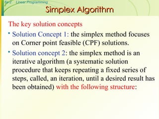
Initialization: setup to start iterations, including
finding an initial CPF solution
Optimality test: is the current CPF solution
optimal?
if no if yes stop
Iteration: Perform an iteration to find a
better CFP solution
4.
6s-4 Linear Programming
Simplexalgorithm
Simplex algorithm
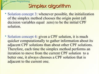
Solution concept 3: whenever possible, the initialization
of the simplex method chooses the origin point (all
decision variables equal zero) to be the initial CPF
solution.
Solution concept 4: given a CPF solution, it is much
quicker computationally to gather information about its
adjacent CPF solutions than about other CPF solutions.
Therefore, each time the simplex method performs an
iteration to move from the current CPF solution to a
better one, it always chooses a CPF solution that is
adjacent to the current one.
5.
6s-5 Linear Programming
Simplexalgorithm
Simplex algorithm
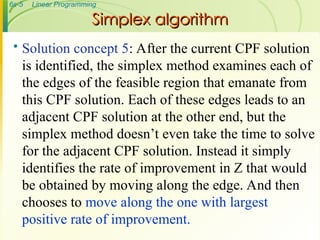
Solution concept 5: After the current CPF solution
is identified, the simplex method examines each of
the edges of the feasible region that emanate from
this CPF solution. Each of these edges leads to an
adjacent CPF solution at the other end, but the
simplex method doesn’t even take the time to solve
for the adjacent CPF solution. Instead it simply
identifies the rate of improvement in Z that would
be obtained by moving along the edge. And then
chooses to move along the one with largest
positive rate of improvement.
6.
6s-6 Linear Programming
Simplexalgorithm
Simplex algorithm
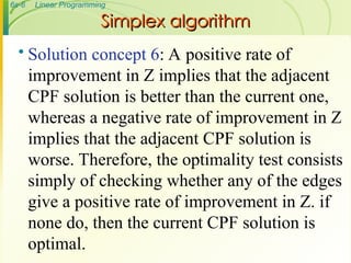
Solution concept 6: A positive rate of
improvement in Z implies that the adjacent
CPF solution is better than the current one,
whereas a negative rate of improvement in Z
implies that the adjacent CPF solution is
worse. Therefore, the optimality test consists
simply of checking whether any of the edges
give a positive rate of improvement in Z. if
none do, then the current CPF solution is
optimal.
7.
6s-7 Linear Programming
Thesimplex method in tabular form
The simplex method in tabular form
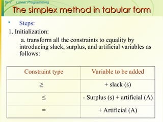
Steps:
1. Initialization:
a. transform all the constraints to equality by
introducing slack, surplus, and artificial variables as
follows:
Constraint type Variable to be added
≥ + slack (s)
≤ - Surplus (s) + artificial (A)
= + Artificial (A)
8.
6s-8 Linear Programming
Simplexmethod in tabular form
Simplex method in tabular form
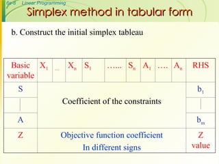
b. Construct the initial simplex tableau
Basic
variable
X1 … Xn S1 …... Sn A1 …. An RHS
S
Coefficient of the constraints
b1
A bm
Z Objective function coefficient
In different signs
Z
value
9.
6s-9 Linear Programming
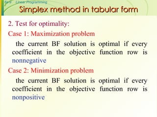
2.Test for optimality:
Case 1: Maximization problem
the current BF solution is optimal if every
coefficient in the objective function row is
nonnegative
Case 2: Minimization problem
the current BF solution is optimal if every
coefficient in the objective function row is
nonpositive
Simplex method in tabular form
Simplex method in tabular form
10.
6s-10 Linear Programming
Simplexmethod in tabular form
Simplex method in tabular form
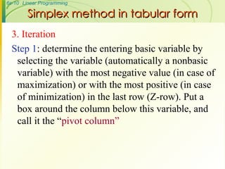
3. Iteration
Step 1: determine the entering basic variable by
selecting the variable (automatically a nonbasic
variable) with the most negative value (in case of
maximization) or with the most positive (in case
of minimization) in the last row (Z-row). Put a
box around the column below this variable, and
call it the “pivot column”
11.
6s-11 Linear Programming
Simplexmethod in tabular form
Simplex method in tabular form
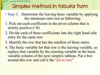
Step 2: Determine the leaving basic variable by applying
the minimum ratio test as following:
1. Pick out each coefficient in the pivot column that is
strictly positive (>0)
2. Divide each of these coefficients into the right hand side
entry for the same row
3. Identify the row that has the smallest of these ratios
4. The basic variable for that row is the leaving variable, so
replace that variable by the entering variable in the basic
variable column of the next simplex tableau. Put a box
around this row and call it the “pivot row”
12.
6s-12 Linear Programming
Simplexmethod in tabular form
Simplex method in tabular form
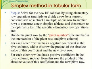
Step 3: Solve for the new BF solution by using elementary
row operations (multiply or divide a row by a nonzero
constant; add or subtract a multiple of one row to another
row) to construct a new simplex tableau, and then return to
the optimality test. The specific elementary row operations
are:
1. Divide the pivot row by the “pivot number” (the number in
the intersection of the pivot row and pivot column)
2. For each other row that has a negative coefficient in the
pivot column, add to this row the product of the absolute
value of this coefficient and the new pivot row.
3. For each other row that has a positive coefficient in the
pivot column, subtract from this row the product of the
absolute value of this coefficient and the new pivot row.
13.
6s-13 Linear Programming
Simplexmethod
Simplex method
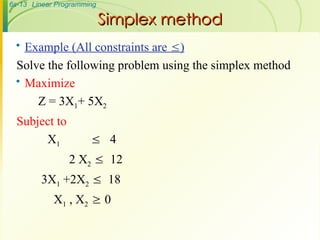
Example (All constraints are )
Solve the following problem using the simplex method
Maximize
Z = 3X1+ 5X2
Subject to
X1 4
2 X2 12
3X1 +2X2 18
X1 , X2 0
14.
6s-14 Linear Programming
Simplexmethod
Simplex method
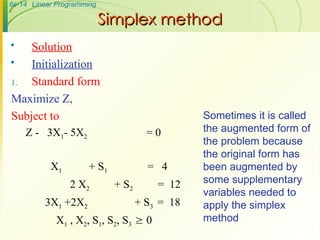
Solution
Initialization
1. Standard form
Maximize Z,
Subject to
Z - 3X1- 5X2 = 0
X1 + S1 = 4
2 X2 + S2 = 12
3X1 +2X2 + S3 = 18
X1 , X2, S1, S2, S3 0
Sometimes it is called
the augmented form of
the problem because
the original form has
been augmented by
some supplementary
variables needed to
apply the simplex
method
15.
6s-15 Linear Programming
Definitions
Definitions
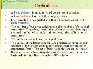
A basic solution is an augmented corner point solution.
A basic solution has the following properties:
1. Each variable is designated as either a nonbasic variable or a
basic variable.
2. The number of basic variables equals the number of functional
constraints. Therefore, the number of nonbasic variables equals
the total number of variables minus the number of functional
constraints.
3. The nonbasic variables are set equal to zero.
4. The values of the basic variables are obtained as simultaneous
solution of the system of equations (functional constraints in
augmented form). The set of basic variables are called “basis”
5. If the basic variables satisfy the nonnegativity constraints, the
basic solution is a Basic Feasible (BF) solution.
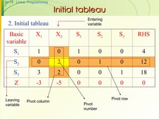
6s-17 Linear Programming
Simplextableau
Simplex tableau
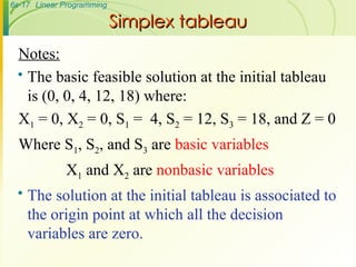
Notes:
The basic feasible solution at the initial tableau
is (0, 0, 4, 12, 18) where:
X1 = 0, X2 = 0, S1 = 4, S2 = 12, S3 = 18, and Z = 0
Where S1, S2, and S3 are basic variables
X1 and X2 are nonbasic variables
The solution at the initial tableau is associated to
the origin point at which all the decision
variables are zero.
18.
6s-18 Linear Programming
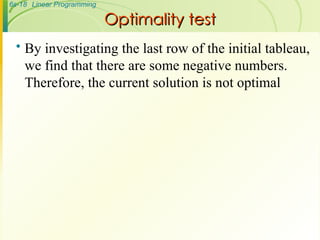
Optimalitytest
Optimality test
By investigating the last row of the initial tableau,
we find that there are some negative numbers.
Therefore, the current solution is not optimal
19.
6s-19 Linear Programming
Iteration
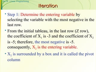
Iteration
Step 1: Determine the entering variable by
selecting the variable with the most negative in the
last row.
From the initial tableau, in the last row (Z row),
the coefficient of X1 is -3 and the coefficient of X2
is -5; therefore, the most negative is -5.
consequently, X2 is the entering variable.
X2 is surrounded by a box and it is called the pivot
column
20.
6s-20 Linear Programming
Iteration
Iteration
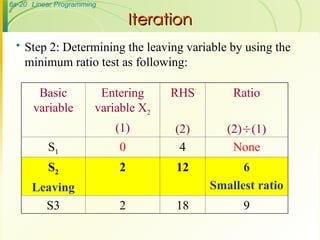
Step 2: Determining the leaving variable by using the
minimum ratio test as following:
Basic
variable
Entering
variable X2
(1)
RHS
(2)
Ratio
(2)(1)
S1 0 4 None
S2
Leaving
2 12 6
Smallest ratio
S3 2 18 9
21.
6s-21 Linear Programming
Iteration
Iteration
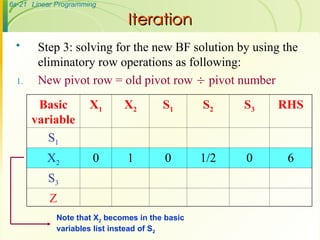
Step 3: solving for the new BF solution by using the
eliminatory row operations as following:
1. New pivot row = old pivot row pivot number
Basic
variable
X1 X2 S1 S2 S3 RHS
S1
X2 0 1 0 1/2 0 6
S3
Z
Note that X2 becomes in the basic
variables list instead of S2
22.
6s-22 Linear Programming
iteration
iteration
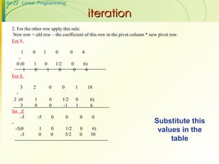
2.For the other row apply this rule:
New row = old row – the coefficient of this row in the pivot column * new pivot row.
For S1
1 0 1 0 0 4
-
0 (0 1 0 1/2 0 6)
1 0 1 0 0 4
For S3
3 2 0 0 1 18
-
2 (0 1 0 1/2 0 6)
3 0 0 -1 1 6
for Z
-3 -5 0 0 0 0
-
-5(0 1 0 1/2 0 6)
-3 0 0 5/2 0 30
Substitute this
values in the
table
23.
6s-23 Linear Programming
Iteration
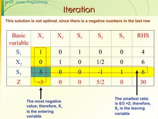
Iteration
Basic
variable
X1X2 S1 S2 S3 RHS
S1 1 0 1 0 0 4
X2 0 1 0 1/2 0 6
S3 3 0 0 -1 1 6
Z -3 0 0 5/2 0 30
The most negative
value; therefore, X1
is the entering
variable
The smallest ratio
is 6/3 =2; therefore,
S3 is the leaving
variable
This solution is not optimal, since there is a negative numbers in the last row
24.
6s-24 Linear Programming
Iteration
Iteration
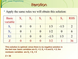
Apply the same rules we will obtain this solution:
Basic
variable
X1 X2 S1 S2 S3 RHS
S1 0 0 1 1/3 -1/3 2
X2 0 1 0 1/2 0 6
X1 1 0 0 -1/3 1/3 2
Z 0 0 0 3/2 1 36
This solution is optimal; since there is no negative solution in
the last row: basic variables are X1 = 2, X2 = 6 and S1 = 2; the
nonbasic variables are S2 = S3 = 0
Z = 36
25.
6s-25 Linear Programming
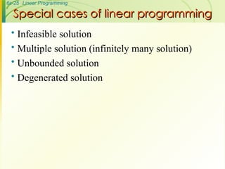
Specialcases of linear programming
Special cases of linear programming
Infeasible solution
Multiple solution (infinitely many solution)
Unbounded solution
Degenerated solution