Download as PDF, PPTX

![Machine Learning
Srihari
Notation
• N observations of x
x = (x1,..,xN)T
t = (t1,..,tN)T
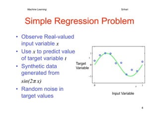
• Goal is to exploit training
set to predict value of
from x
Data Generation:
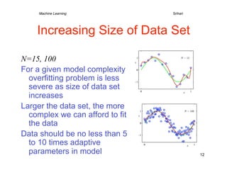
• Inherently a difficult N = 10
problem Spaced uniformly in range [0,1]
Generated from sin(2πx) by adding
• Probability theory allows small Gaussian noise
us to make a prediction Noise typical due to unobserved variables
5](https://image.slidesharecdn.com/curve-fitting-121217135153-phpapp02/85/Curve-fitting-5-320.jpg)
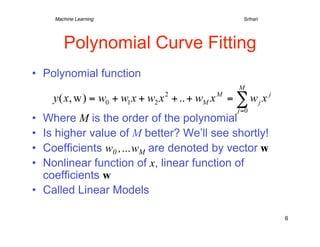
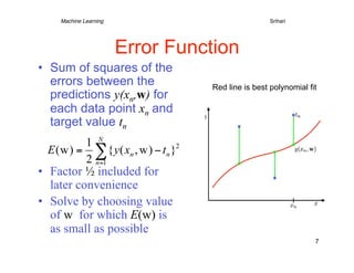
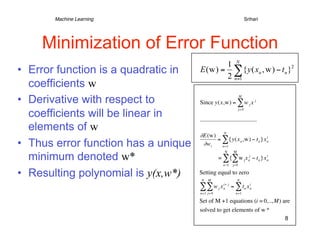
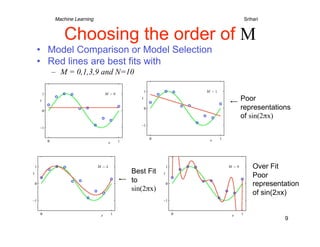

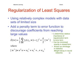
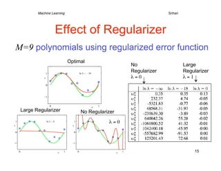
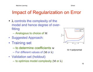

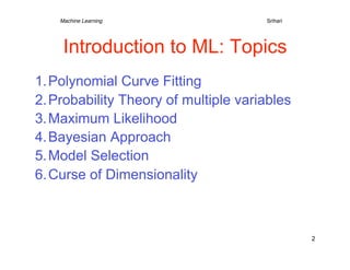
1) The document discusses machine learning concepts including polynomial curve fitting, probability theory, maximum likelihood, Bayesian approaches, and model selection. 2) It describes using polynomial functions to fit a curve to data points and minimizing the error between predictions and actual target values. Higher order polynomials can overfit noise in the data. 3) Regularization is introduced to add a penalty for high coefficient values in complex models to reduce overfitting, analogous to limiting the polynomial order. This improves generalization to new data.


![Cmmi hm 2008 sepg model changes for high maturity 1v01[1]](https://cdn.slidesharecdn.com/ss_thumbnails/cmmihm2008sepgmodelchangesforhighmaturity1v011-150525024656-lva1-app6892-thumbnail.jpg?width=640&height=640&fit=bounds)
![Cmmi%20 model%20changes%20for%20high%20maturity%20v01[1]](https://cdn.slidesharecdn.com/ss_thumbnails/cmmi20model20changes20for20high20maturity20v011-150525024513-lva1-app6892-thumbnail.jpg?width=640&height=640&fit=bounds)


![Introduction to bayesian_networks[1]](https://cdn.slidesharecdn.com/ss_thumbnails/introductiontobayesiannetworks1-150525024327-lva1-app6891-thumbnail.jpg?width=640&height=640&fit=bounds)
![Workshop healthy ingredients ppm[1]](https://cdn.slidesharecdn.com/ss_thumbnails/workshophealthy-ingredientsppm1-150525024135-lva1-app6892-thumbnail.jpg?width=640&height=640&fit=bounds)


