Module10 the regression analysis

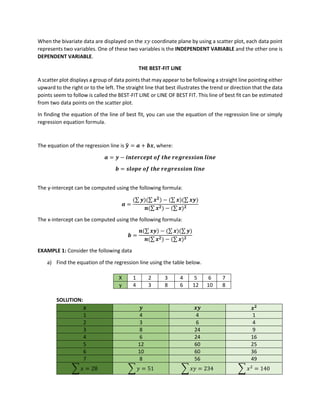
1. When the bivariate data are displayed on the 𝑥𝑦 coordinate plane by using a scatter plot, each data point
represents two variables. One of these two variables is the INDEPENDENT VARIABLE and the other one is
DEPENDENT VARIABLE.
THE BEST-FIT LINE
A scatter plot displays a group of data points that may appear to be following a straight line pointing either
upward to the right or to the left. The straight line that best illustrates the trend or direction that the data
points seem to follow is called the BEST-FIT LINE or LINE OF BEST FIT. This line of best fit can be estimated
from two data points on the scatter plot.
In finding the equation of the line of best fit, you can use the equation of the regression line or simply
regression equation formula.
The equation of the regression line is 𝒚
̂ = 𝒂 + 𝒃𝒙, where:
𝒂 = 𝒚 − 𝒊𝒏𝒕𝒆𝒓𝒄𝒆𝒑𝒕 𝒐𝒇 𝒕𝒉𝒆 𝒓𝒆𝒈𝒓𝒆𝒔𝒔𝒊𝒐𝒏 𝒍𝒊𝒏𝒆
𝒃 = 𝒔𝒍𝒐𝒑𝒆 𝒐𝒇 𝒕𝒉𝒆 𝒓𝒆𝒈𝒓𝒆𝒔𝒔𝒊𝒐𝒏 𝒍𝒊𝒏𝒆
The y-intercept can be computed using the following formula:
𝒂 =
(∑ 𝒚)(∑ 𝒙𝟐
) − (∑ 𝒙)(∑ 𝒙𝒚)
𝒏(∑ 𝒙𝟐) − (∑ 𝒙)𝟐
The x-intercept can be computed using the following formula:
𝒃 =
𝒏(∑ 𝒙𝒚) − (∑ 𝒙)(∑ 𝒚)
𝒏(∑ 𝒙𝟐) − (∑ 𝒙)𝟐
EXAMPLE 1: Consider the following data
a) Find the equation of the regression line using the table below.
X 1 2 3 4 5 6 7
y 4 3 8 6 12 10 8
SOLUTION:
𝒙 𝒚 𝒙𝒚 𝒙𝟐
1 4 4 1
2 3 6 4
3 8 24 9
4 6 24 16
5 12 60 25
6 10 60 36
7 8 56 49
∑ 𝑥 = 28 ∑ 𝑦 = 51 ∑ 𝑥𝑦 = 234 ∑ 𝑥2
= 140

2. The y-intercept can be computed using the following formula:
𝒂 =
(∑ 𝒚)(∑ 𝒙𝟐
) − (∑ 𝒙)(∑ 𝒙𝒚)
𝒏(∑ 𝒙𝟐) − (∑ 𝒙)𝟐
𝒂 =
(𝟓𝟏)(𝟏𝟒𝟎) − (𝟐𝟖)(𝟐𝟑𝟒)
𝟕(𝟏𝟒𝟎) − (𝟐𝟖)𝟐
=
𝟕, 𝟏𝟒𝟎 − 𝟔, 𝟓𝟓𝟐
𝟗𝟖𝟎 − 𝟕𝟖𝟒
=
𝟓𝟖𝟖
𝟏𝟗𝟔
= 𝟑
The x-intercept can be computed using the following formula:
𝒃 =
𝒏(∑ 𝒙𝒚) − (∑ 𝒙)(∑ 𝒚)
𝒏(∑ 𝒙𝟐) − (∑ 𝒙)𝟐
𝒃 =
𝟕(𝟐𝟑𝟒) − (𝟐𝟖)(𝟓𝟏)
𝟕(𝟏𝟒𝟎) − (𝟐𝟖)𝟐
=
𝟏, 𝟔𝟑𝟖 − 𝟏, 𝟒𝟐𝟖
𝟗𝟖𝟎 − 𝟕𝟖𝟒
=
𝟐𝟏𝟎
𝟏𝟗𝟔
= 𝟏. 𝟎𝟕𝟏𝟒𝟐 𝒐𝒓 𝟏. 𝟎𝟕𝟏
The equation of the regression line is
𝒚
̂ = 𝒂 + 𝒃𝒙
𝒚
̂ = 𝟑 + 𝟏. 𝟎𝟕𝟏𝒙
EXAMPLE 2: The grades of 7 students in the first and second grading periods are shown below.
a) Find the equation of the regression line.
b) Estimate the grade in the second grading period of a student who received a grade of 88 in
the first grading period.
x 80 78 76 82 84 85 75
y 84 79 75 86 84 77 78
SOLUTION:
𝒙 𝒚 𝒙𝒚 𝒙𝟐
80 84 6,720 6,400
78 79 6,162 6,084
76 75 5,700 5,776
82 86 7,052 6,724
84 84 7,056 7,056
85 77 6,545 7,225
75 78 5,850 5,625
∑ 𝒙 = 𝟓𝟔𝟎 ∑ 𝒚 = 𝟓𝟔𝟑 ∑ 𝒙𝒚 = 𝟒𝟓, 𝟎𝟖𝟓 ∑ 𝒙𝟐
= 𝟒𝟒, 𝟖𝟗𝟎
The y-intercept can be computed using the following formula:
𝒂 =
(∑ 𝒚)(∑ 𝒙𝟐
) − (∑ 𝒙)(∑ 𝒙𝒚)
𝒏(∑ 𝒙𝟐) − (∑ 𝒙)𝟐

3. 𝒂 =
(𝟓𝟔𝟑)(𝟒𝟒, 𝟖𝟗𝟎) − (𝟓𝟔𝟎)(𝟒𝟓, 𝟎𝟖𝟓)
𝟕(𝟒𝟒, 𝟖𝟗𝟎) − (𝟓𝟔𝟎)𝟐
=
𝟐𝟓, 𝟐𝟕𝟑, 𝟎𝟕𝟎 − 𝟐𝟓, 𝟐𝟒𝟕, 𝟔𝟎𝟎
𝟑𝟏𝟒, 𝟐𝟑𝟎 − 𝟑𝟏𝟑, 𝟔𝟎𝟎
=
𝟐𝟓, 𝟒𝟕𝟎
𝟔𝟑𝟎
= 𝟒𝟎. 𝟒𝟐𝟗
The x-intercept can be computed using the following formula:
𝒃 =
𝒏(∑ 𝒙𝒚) − (∑ 𝒙)(∑ 𝒚)
𝒏(∑ 𝒙𝟐) − (∑ 𝒙)𝟐
𝒃 =
𝟕(𝟒𝟓, 𝟎𝟖𝟓) − (𝟓𝟔𝟎)(𝟓𝟔𝟑)
𝟕(𝟒𝟒, 𝟖𝟗𝟎) − (𝟓𝟔𝟎)𝟐
=
𝟑𝟏𝟓, 𝟓𝟗𝟓 − 𝟑𝟏𝟓, 𝟐𝟖𝟎
𝟑𝟏𝟒, 𝟐𝟑𝟎 − 𝟑𝟏𝟑, 𝟔𝟎𝟎
=
𝟑𝟏𝟓
𝟔𝟑𝟎
= 𝟎. 𝟓
The equation of the regression line is
𝒚
̂ = 𝒂 + 𝒃𝒙
𝒚
̂ = 𝟒𝟎. 𝟒𝟐𝟗 + 𝟎. 𝟓𝒙
Estimate the grade in the second grading period of a student who received a grade of 88 in the first grading
period:
𝒚
̂ = 𝟒𝟎. 𝟒𝟐𝟗 + 𝟎. 𝟓𝒙
𝒚
̂ = 𝟒𝟎. 𝟒𝟐𝟗 + 𝟎. 𝟓(𝟖𝟖)
𝒚
̂ = 𝟒𝟎. 𝟒𝟐𝟗 + 𝟒𝟒
𝒚
̂ = 𝟖𝟒. 𝟒𝟐𝟗 𝒐𝒓 𝟖𝟒. 𝟒𝟑
A student whose grade is 88 in the first grading can expect a grade of 84.43 in the second grading.