Study of consolidation parameters

STUDY OF CONSOLIDATION
PARAMETERS
MEHAK AGGARWAL
M.PHARM (PHARMACEUTICS)
HIMACHAL INSTITUTE OF PHARMACY

CONTENT
• Consolidation
• Diffusion parameters
• Dissolution parameters
• Pharmacokinetic parameters
• Similarity factors f1 and f2
• Heckel plots
• Higuchi equation
• Korsmeyer-peppas plot
• Linearity concept of significance
• Standard deviation
• Chi square test
• Student t-test
• ANOVA test
• References
1/24/2022
MEHAK AGGARWAL 2

CONSOLIDATION
An increase in the mechanical strength of the material resulting from particle-particle
interaction. (Increasing in mechanical strength of the mass).
CONSOLIDATION PROCESS
• Cold welding:
When the surfaces of two particles approach each other closely enough, their free
surface energies results in strong attractive force, a process known as cold welding.
• Fusion bonding:
Multiple point contacts of the particle upon application of load produces heat which
causes fusion / melting. Upon removal of load it gets solidified and increase the
mechanical strength of mass.
1/24/2022
MEHAK AGGARWAL 3

CONSOLIDATION MECHANISMS
1. Mechanical theory:
• As the particles undergo deformation, the particle boundaries that the edges of the
particle intermesh, forming a mechanical bond.
2. Intermolecular forces theory:
• Under pressure the molecules at the point of true contact between new, clean
surface of the granules are close enough so that van der Waals forces interact to
consolidate the particle.
3. Liquid-surface film theory:
• Thin liquid films form bond between the particles which binds them together at the
particle surface. The energy of compression produces melting of solution at the
particle interface followed by subsequent solidification or crystallization thus
resulting in the formation of bonded surfaces.
1/24/2022
MEHAK AGGARWAL 4

FACTORS AFFECTING CONSOLIDATION:
• The chemical nature of the material
• The extent of the available surface
• The presence of surface contaminants
• The inter surface distance
1/24/2022
MEHAK AGGARWAL 5

DIFFUSION PARAMETERS
• This is given by Higuchi.
𝑄 = 𝐾√𝑻
Where,
Q is the amount of drug released in time ‘t’ per unit area
K is higuchi constant
T is time in hr.
• Plot: The data obtained is to be plotted as cumulative percentage drug release versus
Square root of time.
• Application: modified release pharmaceutical dosage forms, transdermal systems and
matrix tablets with water soluble drugs.
1/24/2022
MEHAK AGGARWAL 6

DISSOLUTION PARAMETERS
• Dissolution is a process in which a solid substance solubilizes in a given solvent i.e. mass transfer
from the solid surface to the liquid phase.
• Dissolution parameters:
 Effect of agitation
 Effect of dissolution fluid
 Influence of pH of dissolution fluid
 Effect of viscosity of the dissolution medium
 Effect of the presence of unreactive and reactive additives in the dissolution medium.
 Volume of dissolution medium and sink conditions
 Deaeration of the dissolution medium
 Effect of temperature of the dissolution medium
MEHAK AGGARWAL 1/24/2022 7

EFFECT OF AGITATION
• The relationship between the intensity of agitation and the rate of dissolution varies
considerably according to the type of agitation used, the shape and design of the
stirrer and the physicochemical properties of the solid.
• For the basket method, 100 rpm usually is utilized, while for the paddle procedure, a
50 – 75 rpm is recommended.
EFFECT OF DISSOLUTION FLUID
• Selection of proper medium for dissolution testing depends largely on the
physicochemical properties of the drug.
INFLUENCE OF PH OF DISSOLUTION FLUID
• Simulated gastric fluid as the test medium for tablets containing ingredients which
reacted more readily in acid solution than in water (e.g., calcium carbonate).

EFFECT OF VISCOSITY OF THE DISSOLUTION MEDIUM
• If the interaction at the interfaces, occurs much faster than the rate of transport,
such as in the case of diffusion controlled dissolution processes, it would be
expected that the dissolution rate decreases with an increase in viscosity.
• The rate of dissolution of zinc in HCl solution containing sucrose was inversely
proportional to the viscosity of solution.
EFFECT OF THE PRESENCE OF UNREACTIVE AND REACTIVE ADDITIVES IN THE
DISSOLUTION MEDIUM
• When neutral ionic compounds, such as sodium chloride and sodium sulfate, or non
ionic organic compounds, such as dextrose, were added to the dissolution medium,
the dissolution of benzoic acid was dependent linearly upon its solubility in the
particular solvent.
• When certain buffers or bases were added to the aqueous solvent , an increase in the
dissolution rate was observed.

VOLUME OF DISSOLUTION MEDIUM AND SINK CONDITIONS
• The proper volume of the dissolution medium depends mainly on the solubility of the drug in the
selected fluid.
• If the drug is poorly soluble in water, a relatively large amount of fluid should be used if complete
dissolution is to be expected.
DEAERATION OF THE DISSOLUTION MEDIUM
• Presence of dissolved air or other gases in the dissolution medium may influence the dissolution
rate of certain formulations and lead to variable and unreliable results.
• Example, the dissolved air in distilled water could significantly lower its pH and consequently affect
the dissolution rate of drugs that are sensitive to pH changes, e.g., weak acids.
EFFECT OF TEMPERATURE OF THE DISSOLUTION MEDIUM
• Drug solubility is temperature dependent, therefore careful temperature control during the
dissolution process is extremely important.
• Generally a temperature of 37°±0.5 is maintained during dissolution determination of oral dosage
forms and suppositories.
• For topical preparations as low as 30° and 25°have been used.

PHARMACOKINETIC PARAMETERS
• Pharmacokinetics is defined as the kinetics of drug absorption, distribution,
metabolism, and excretion and their relationship with pharmacologic, therapeutic or
toxicologic response in mans and animals.
PLASMA DRUG CONCENTRATION TIME PROFILE

Three important pharmacokinetic parameters:
1. Peak plasma concentration (Cmax)
2. Time of peak concentration (tmax)
3. Area under the curve (AUC)
PEAK PLASMA CONCENTRATION (Cmax)
• The point of maximum concentration of a drug in plasma is called as peak and the
concentration of drug at peak is known as peak plasma concentration.
• It is also called as peak height concentration and maximum drug concentration.
• Cmax is expressed in mcg/ml.

TIME OF PEAK CONCENTRATION (tmax)
• The time for drug to reach peak concentration in plasma ( after extravascular
administration) is called the time of peak concentration.
• It is expressed in hours.
AREA UNDER THE CURVE (AUC)
• It represents the total integrated area under the plasma level- time profile and
expresses the total amount of drug that comes into the systemic circulation after its
administration.
• AUC is expressed in mcg/ml X HRS.
• It is important for the dugs that are administered repetitively for the treatment of
chronic conditions like asthma or epilepsy.

SIMILARITY FACTORS F1 AND F2
DIFFERENCE FACTOR (f1)
• The difference factor (f1) as defined by FDA calculates the % difference between 2 curves
at each time point and is a measurement of the relative error between 2 curves.
SIMILARITY FACTOR (f2)
• The similarity factor (f2 ) is a logarithmic reciprocal square root transformation of the
sum of squared error and is a measurement of the similarity in the percent (%)
dissolution between the two curves.
where, n = number of time points, Rt = % dissolved at time t of reference product (pre change),
Tt = % dissolved at time t of test product (post change)

APPLICATIONS OF f1
• F1 is specially used to compare two dissolution profiles, being necessary to consider
one of them as the reference standard product.
• It can measure the percent of error between two curves over all time points.
APPLICATIONS OF f2
• This method is more appropriate when more than three or four dissolution time
points are available.
• The f2 may become invariant with respect to the location change and the
consequence of failure to take into account the shape of the curve and the unequal
spacing between sampling time points lead to errors.
• Nevertheless, with a slight modification in the statistical analysis, similarity factor
would definitely serves as an efficient tool for reliable comparison of dissolution
profiles.

Advantages
1. They are easy to compute.
2. They provide a single number to describe the comparison of dissolution profile
data.
Disadvantages
1. The values of f1 and f2 are sensitive to the number of dissolution time points used.
2. The basis of the criteria for deciding the difference or similarity between
dissolution profile is unclear.

HECKEL PLOTS
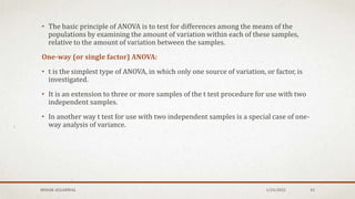
• The Heckel analysis is a most popular method of deforming reduction under
pressure.
• It is based upon analogous behavior to first order reaction where the pores in the
mass are the reactant, i.e.,
Log 1/E=Ky . P+Kr
where,
Ky=material dependent constant but inversely proportional to its yield strength(S)
Kr=related packing stage [E0].

The applied compressional force F & the movement of the punches during
compression cycle & applied pressure P , porosity E.
For a cylindrical tablets
p=4F/л. D2
Where, D is the tablet diameter similarly E can be calculated by
E=100.(1-4w/ρt .л.D2.H)
Where, w is the weight of the tableting mass ,
ρt is its true density ,
H is the thickness of the tab

• Based on Heckel Equation there are 3 types of powders:-
1. TYPE-A
2. TYPE-B
3. TYPE-C
• FOR TYPE-A MATERIAL:
A linear relationship is observed, with the plots remaining parallel as the applied
pressure is increased indicating deformation apparently only by plastic deformation.
Soft materials undergo plastic deformation readily and retain different degree of
porosity, depending upon the initial packing of die. Thus, in turn influenced by the size
distribution, shape etc., of the original particles.
e.g.:-Sodium chloride

• FOR TYPE-B MATERIALS:
There is an initial curved region followed by a straight line. This indicates that the
particles are fragmenting at the early stages of the compression process.
Harder materials with higher yield pressure values usually undergo compression by
fragmentation first, to provide a denser packing.
e.g. : Lactose; Sucrose.
• FOR TYPE-C MATERIALS:
There is an initial step linear region which become superimposed and flatten out as
applied pressure is increased. T
his behavior to the absence of a rearrangement stage and densification is due to plastic
deformation and asperity melting.

• Type-A plots, exhibits higher slope(Ky) than type-b, because type-a have lower yield
stress than type-a.
• Type-B plots, exhibits lower slope(Ky)because brittle, hard materials are difficult to
compress.

• Heckel plot is density Vs applied pressure and it follows first order kinetics.
• As porosity increases compression force also increases.
• Thus, Heckel plot allows for the interpretation of the mechanical bonding and it also
identifies the predominant form of deformation for a given sample.
• Heckel plot represent in two regions:
1. Initial repacking stage.
2. Subsequent deformation process.
LIMITATIONS:
Heckel plot is influenced by;
1. Degree of lubrication.
2. Size of the die.
3. Residual porosity in particular formulations provide good mechanical strength, rapid
water intake and hence good disintegration characteristics.

APPLICATION OF HECKEL EQUATION
• The crushing strength of tablets can be correlated with the values of k of the Heckel
plot .
• Larger k values usually indicate harder tablets.
• Such information can be used as a means of binder selection when designing tablet
formulations.
• Heckel plots can be influenced by the overall time of compression, the degree of
lubrication and even the size of the die, so that the effects of these variables are also
important and should be taken into consideration

HIGUCHI EQUATION (DIFFUSION MATRIX FORMULATION)
• Higuchi proposed this model in 1961 to describe drug release from matrix system. It is
developed to study the water soluble and low soluble drugs incorporated in semisolids
and solid matrices.
• It is based on the hypothesis that;
1. Initial drug concentration in the matrix is much higher than drug solubility.
2. Drug diffusion takes place in only one direction (edge effect must be negligible).
3. Drug particles are much smaller than system thickness.
4. Matrix swelling and dissolution are negligible.
5. Drug diffusivity is constant.
6. Perfect sink conditions are always attained in the release environment.

• Higuchi model is given by
where,
Q= Amount of drug released in time ‘t’ per unit area.
K= Higuchi constant.
T= Time (in hours).
C= Initial frug concentration
Cs= Drug solubility in matrix media.
D= Diffusivity of drug molecules in solvent.

PLOT:
• The data obtained were plotted as cumulative percentage drug release Vs square
root of time.
APPLICATIONS:
• Modified release pharmaceutical dosage forms , transdermal systems and matrix
tablets with water soluble drugs.

KORSMEYER - PEPPAS PLOT
• The KORSEMEYER AND PEPPAS described this method.
• It is given by the equation :
Mt /M∞ = Ktn
Where,
Mt / M ∞ is fraction of drug released
t = time K=constant includes structural and geometrical characteristics of the dosage form
n= release component which is indicative of drug release mechanism where , n is diffusion
exponent.
• If n= 1 , the release is zero order, n = 0.5 the release is best described by the Fickian
diffusion 0.5 < n < 1 then release is through anomalous diffusion or case two diffusion.
• In this model a plot of percent drug release versus time is linear.

PLOT:
• The data obtained were plotted as log cumulative percentage drug release Vs log time.
APPLICATIONS:
• It is applicable to linearization of release data from microcapsules and microspheres.

LINEARITY CONCEPT OF SIGNIFICANCE
• Tests of statistical significance are invariably applied now-a-days by research
scientists. Good medical journals refuse to accept papers for publication if the
authors have not used the philosophy of significance testing in evaluating their
results.
• It is not adequate to mechanically undertake significance tests , the
scientists/experimental workers must fully understand the basic concepts
underlying a significance test, the assumptions involved and the limitations, for
making the proper interpretations.
• Generally, the existence of statistical significance difference is regarded as a proof of
the existence of an important difference between two sample results. Similarly, the
non-significant differences are regarded as proof of no differences in two sample
results.

STANDARD DEVIATION
• Standard Deviation is a number that describes how much data vary or spread out.
• It uses difference of each data value from the mean.
• The higher the number, more data is spread out.
• Finding Standard Deviation
1. Find the mean,
2. Find the difference of each data value from the mean,
3. Square each difference

4. Sum all the squared values
5. Divide by the number of data taken by the sample minus 1.
6. Take the square root

CHI-SQUARE TEST
• The chi-square test is an important test amongst the several tests of significance
developed by statisticians.
• It was developed by Karl Pearson in 1900.
• CHI SQUARE TEST is a non parametric test not based on any assumption or
distribution of any variable.
• This statistical test follows a specific distribution known as chi square distribution.
• In general, the test we use to measure the differences between what is observed and
what is expected according to an assumed hypothesis is called the chi-square test.

Chi-Square as a Parametric Test
Test for comparing variance
Chi-Square as a Non-Parametric Test
• Test of Goodness of Fit
• Test of Independence
Where, O= observed frequencies
E= expected frequency

AS A TEST OF GOODNESS OF FIT
• It enables us to see how well does the assumed theoretical distribution (such as Binomial
distribution, Poisson distribution or Normal distribution) fit to the observed data. When
the calculated value of χ2 is less than the table value at certain level of significance, the fit
is considered to be good one and if the calculated value is greater than the table value,
the fit is not considered to be good.
AS A TEST OF INDEPENDENCE
• χ2 test enables us to explain whether or not two attributes are associated. Testing
independence determines whether two or more observations across two populations are
dependent on each other (i.e., whether one variable helps to estimate the other). If the
calculated value is less than the table value at certain level of significance for a given
degree of freedom, we conclude that null hypotheses stands which means that two
attributes are independent or not associated. If calculated value is greater than the table
value, we reject the null hypotheses.

Steps involved are:
1. Determine The Hypothesis:
• Ho : The two variables are independent
• Ha : The two variables are associated
2. Calculate Expected frequency
3. Calculate test statistic

4. Determine degree of Freedom
Df= (R-1)(C-1)
Where, R= number of levels in row variable and C= number of levels in column
variable.
5. Compare computed test statistic against a tabled/critical value
The computed value of the Pearson chi-square statistic is compared with the critical
value to determine if the computed value is improbable The critical tabled values are
based on sampling distributions of the Pearson chi-square statistic. If calculated χ2 is
greater than the χ2 table value, reject Ho.

STUDENT’S t- test
• The test is used to compare samples from two different batches.
• It is usually used with small (<30) samples that are normally distributed.
• Types of “t” test are:
• Single sample t test – we have only 1 group; want to test against a hypothetical
mean.
• Independent samples t test – we have 2 means, 2 groups; no relation between
groups, E.g.: When we want to compare the mean of T/T group with Placebo group.
• Paired t test – It consists of samples of matched pairs of similar units or one group of
units tested twice. E.g.: Difference of mean pre & post drug intervention.

• Equation for a one-sample t-test
Where, t= the t statistic
x̄= the mean of the sample
µ= the comparison mean
s= the sample standard deviation
n= the sample size

• Equation for the Independent samples t-test
The independent samples t-test procedure compares means for two groups of cases.

Paired t-test
• A paired t-test is used to compare two population means where you have two
samples in which observations in one sample can be paired with observations in the
other sample.
• A comparison of two different methods of measurement or two different treatments
where the measurements/treatments are applied to the same subjects.
• E.g.:
1. pre-test/post-test samples in which a factor is measured before and after an
intervention
2. Cross-over trials in which individuals are randomized to two treatments and then
the same individuals are crossed-over to the alternative treatment
3. Matched samples, in which individuals are matched on personal characteristics
such as age and sex

• Suppose a sample of “n” subjects were given an antihypertensive drug we want to
check blood pressure before and after treatment . We want to find out the
effectiveness of the treatment by comparing mean pre & post t/t.
• To test the null hypothesis that the true mean difference is zero, the procedure is as
follows:
1. Calculate the difference (di = yi − xi) between the two observations on each pair.
2. Calculate the mean difference, d.
3. Calculate the standard error of the mean differences. S.E=S.D/√n
4. Calculate the t-statistic, which is given by T = d/S.E, Under the null hypothesis, this
statistic follows a t-distribution with n − 1 degrees of freedom.
5. Use tables of the t-distribution to compare your value for T to the tn−1 distribution.
This will give the p-value for the paired t-test.

ANALYSIS OF VARIANCE (ANOVA)
• The analysis of variance(ANOVA) was developed by R. A. Fisher in 1920.
• It is possible to study the significance of the difference of mean values of a large
number of samples at the same time because of ANOVA.
• The ANOVA is classified into two ways:
1. One-way classification
2. Two-way classification
• In one-way classification we take into account the effect of only one variable.
• If there is a two-way classification, the effect of two variables can be studied.

• The basic principle of ANOVA is to test for differences among the means of the
populations by examining the amount of variation within each of these samples,
relative to the amount of variation between the samples.
One-way (or single factor) ANOVA:
• t is the simplest type of ANOVA, in which only one source of variation, or factor, is
investigated.
• It is an extension to three or more samples of the t test procedure for use with two
independent samples.
• In another way t test for use with two independent samples is a special case of one-
way analysis of variance.

The technique involves the following steps:
1. Obtain the mean of each sample i.e.,
2. Find the mean of the sample means:
3. Calculate the sum of squares for variance between the samples (or SS between):

4. Calculate Mean Square (MS) between:
5. Calculate the sum of squares for variance within the samples (or SS within):
6. Calculate Mean Square (MS) within:

7. Calculate SS for total variance:
• SS for total variance = SS between + SS within
• The degrees of freedom for between and within must add up to the degrees of
freedom for total variance i.e.,
1/24/2022
MEHAK AGGARWAL 46

8. Finally, F-ratio may be worked out as under:
• This ratio is used to judge whether the difference among several sample means is
significant or its just a matter of sampling fluctuations.
1/24/2022
MEHAK AGGARWAL 47

Two Way ANOVA
• Two-way ANOVA technique is used when the data are classified on the basis of two
factors.
• For example, the agricultural output may be classified on the basis of different
varieties of seeds and also on the basis of different varieties of fertilizers used.
• It is a statistical test used to determine the effect of two nominal predictor variables
on a continuous outcome variable.
• two-way ANOVA test analyzes the effect of the independent variables on the
expected outcome along with their relationship to the outcome itself.
• two-way design may have repeated measurements of each factor or may not have
repeated values.
1/24/2022
MEHAK AGGARWAL 48

• Types of two-way ANOVA
1. ANOVA technique in context of two-way design when repeated values are not
there.
2. ANOVA technique in context of two-way design when repeated values are there.
ANOVA technique in context of two-way design when repeated values are not there.
• It includes calculation of residual or error variation by subtraction, once we have
calculated the sum of squares for total variance and for variance between varieties of
one treatment as also for variance between varieties of the other treatment.
ANOVA technique in context of two-way design when repeated values are there.
• We can obtain a separate independent measure of inherent or smallest variations.
• Interaction variation: Interaction is the measure of inter relationship among the two
different classifications.
1/24/2022
MEHAK AGGARWAL 49

Graphical method for studying interaction in two-way design.
• For graphs we shall select one of the factors to be used as the x-axis.
• Then we plot the averages for all the samples on the graph and connect the averages
for each variety of other factor by a distinct line.
• If the connecting lines do not cross over each other, then the graph indicates that
there is no interaction.
• But if the lines do cross, they indicate definite interaction or inter-relation between
the two factors.
1/24/2022
MEHAK AGGARWAL 50

The graph indicates that there is a significant interaction because the different
connecting lines for groups of people do cross over each other. We find that A and B
are affected very similarly, but C is affected differently.
1/24/2022
MEHAK AGGARWAL 51

APPLICATIONS OF ANOVA
• Similar to t-test.
• More versatile than t-test.
• ANOVA is the synthesis of several ideas & it is used for multiple purposes.
• The statistical Analysis depends on the design and discussion of ANOVA therefore
includes common statistical designs used in pharmaceutical research.
• In the bioequivalence studies the similarities between the samples will be analyzed
with ANOVA only.
• Pharmacokinetic data also will be evaluated using ANOVA.
• Pharmacodynamics (what drugs does to the body) data also will be analyzed with
ANOVA only.

REFERENCES
1. Hussain L, Ashwini D, Sirish D. (2013). Kinetic modelling and dissolution profiles
comparison: an overview. Int J Pharm Bio Sci. 4(1): 728 - 737.
2.Thomas O’H, Adrian D, Jackie B and John D. (1998). A review of methods used to
compare dissolution profile data. PSTT. 1(5): 214-223.
3.U.S. Department of Health and Human Services Food and Drug Administration
Centre for Drug Evaluation and Research (CDER). (2015). Guidance for industry
dissolution testing of immediate release solid oral dosage forms.
4.Jignesh A, Maulik P, Sachi P. (2015). Comparison of dissolution profile by model
independent & model dependent methods.
1/24/2022
MEHAK AGGARWAL 53

5. Dissolution, bioavailability and bioequivalence by Hamed M. Abdou.
6. The theory and practice of industrial pharmacy by Lachmann Liberman.
7. Biopharmaceutics and pharmacokinetics by D.M. Bhramankar and Sunil b. Jaiswal.
8. Larson G. Martin. (2008). Analysis of Variance. Circulation. 117(1), 115-121.
9. Prabhaker M, Uttam S., Chandra M.P., Priyadarshni M., Gaurav P. (2019).
Application of Student’s t-test, Analysis of Variance and covariance. Ann Card
Anaesth. 22(4), 407-411. https://dx.doi.org/10.4103%2Faca.ACA_94_19
10. Mary L.M. (2013). The Chi-square test of independence. Biochem Med. 23(2), 143-
149. https://dx.doi.org/10.11613%2FBM.2013.018

Study of consolidation parameters

More Related Content

What's hot

Similar to Study of consolidation parameters

More from Mehak AggarwAl

Recently uploaded

Study of consolidation parameters