Downloaded 1,577 times
![Motor Imagery [Hema et al., 2009] I
Motor Imagery is a mental process of a motor action. It includes preparation for movement,
passive observations of action and mental operations of motor representations implicitly or
explicitly. The ability of an individual to control his EEG through imaginary mental tasks enables
him to control devices through a brain machine interface (BMI) or a brain computer interface
(BCI).
The BMI/BCI is a direct communication pathway between the brain and an external device.
BMI/BCIs are often aimed at assisting, augmenting, or repairing human cognitive or
sensory-motor functions. BMI/BCIs are used to rehabilitate people suffering from neuromuscular
disorders as a means of communication or control.
The methodologies of BMI/BCIs can be separated into two approaches:
Invasive (or partially-invasive) BMI/BCIs (ECoG),
Non-invasive BMI/BCIs (EEG, MEG, MRI, fMRI etc).
Invasive and partially-invasive BCIs are accurate. However there are risks of the infection and the
damage. Furthermore, it requires the operation to set the electrodes in the head.
On the other hand, non-invasive BCIs are inferior than invasive BCIs in accuracy, but costs and
risks are very low. Especially, EEG approach is the most studied potential non-invasive interface,
mainly due to its fine temporal resolution, ease of use, portability and low set-up cost.
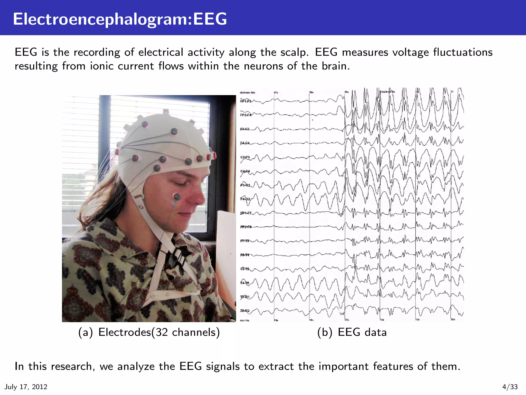
July 17, 2012 3/33](https://image.slidesharecdn.com/main-120718022005-phpapp01/75/Introduction-to-Common-Spatial-Pattern-Filters-for-EEG-Motor-Imagery-Classification-3-2048.jpg)
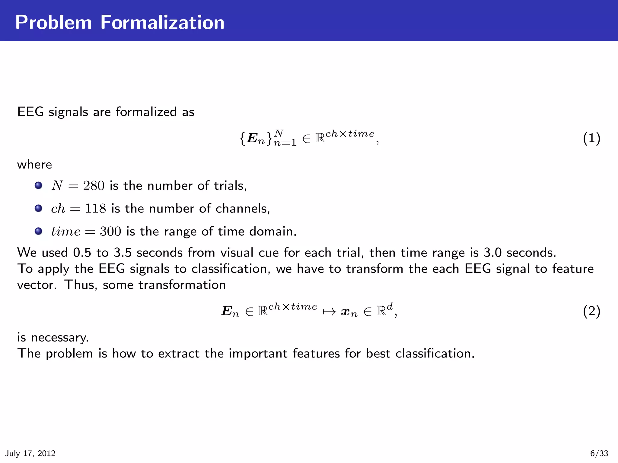
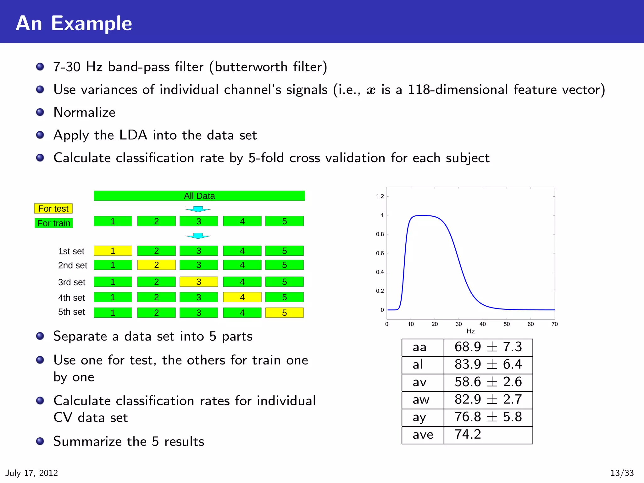
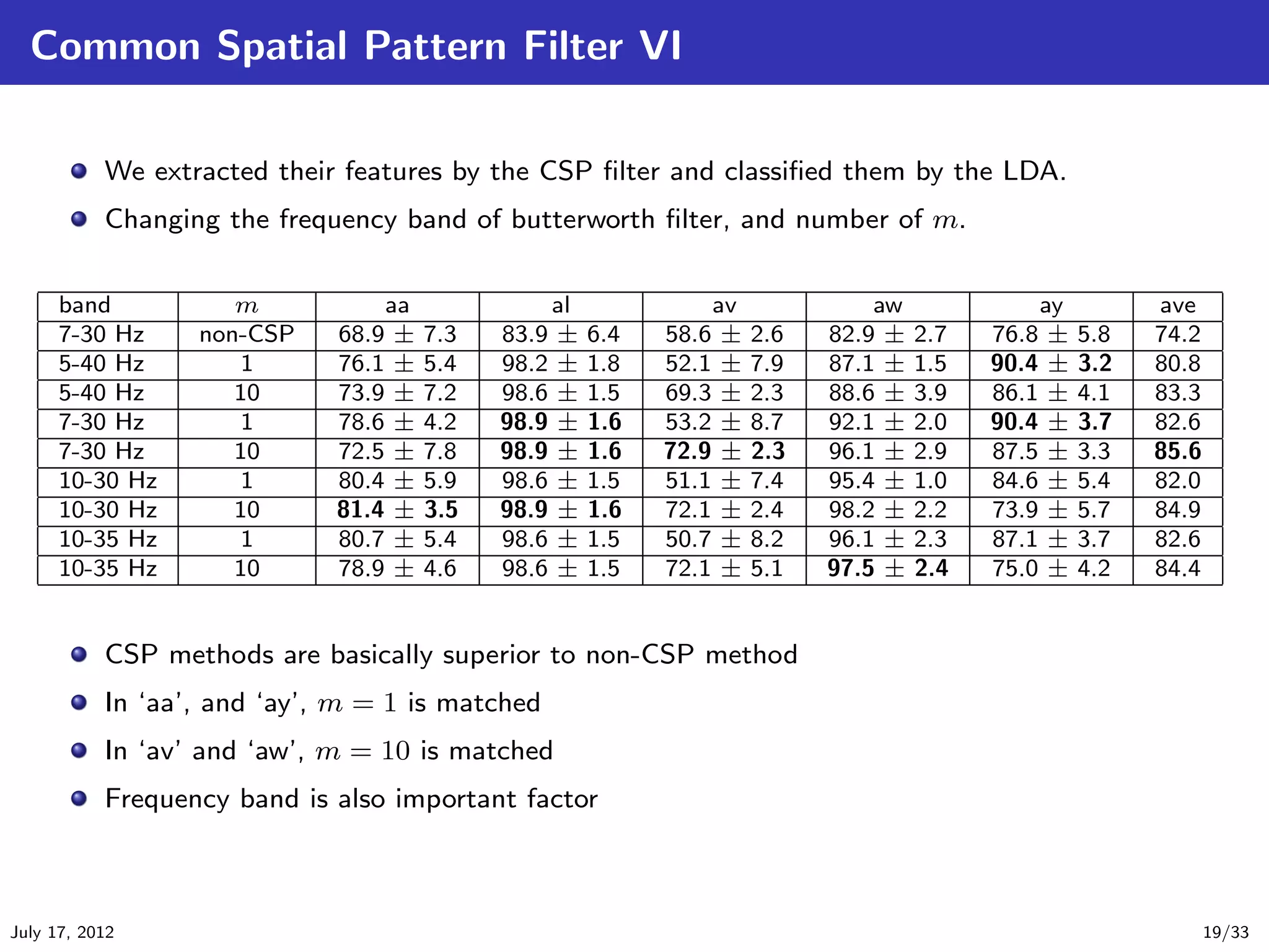
![EEG Motor Imagery Classification
Here, we consider the EEG motor imagery classification problem by BCI competition III
[Blankertz et al., 2006].
Number of subjects is 5 (aa,al,av,aw,ay).
118 channels of electrodes were used.
The problem is to classify the given EEG signal to right hand or right foot.
They recorded their EEG signals for 3.5 seconds with 100 Hz sampling rates for each trial.
For each subject they conducted 280 (hand 140 / foot 140) trials.
July 17, 2012 5/33](https://image.slidesharecdn.com/main-120718022005-phpapp01/75/Introduction-to-Common-Spatial-Pattern-Filters-for-EEG-Motor-Imagery-Classification-5-2048.jpg)
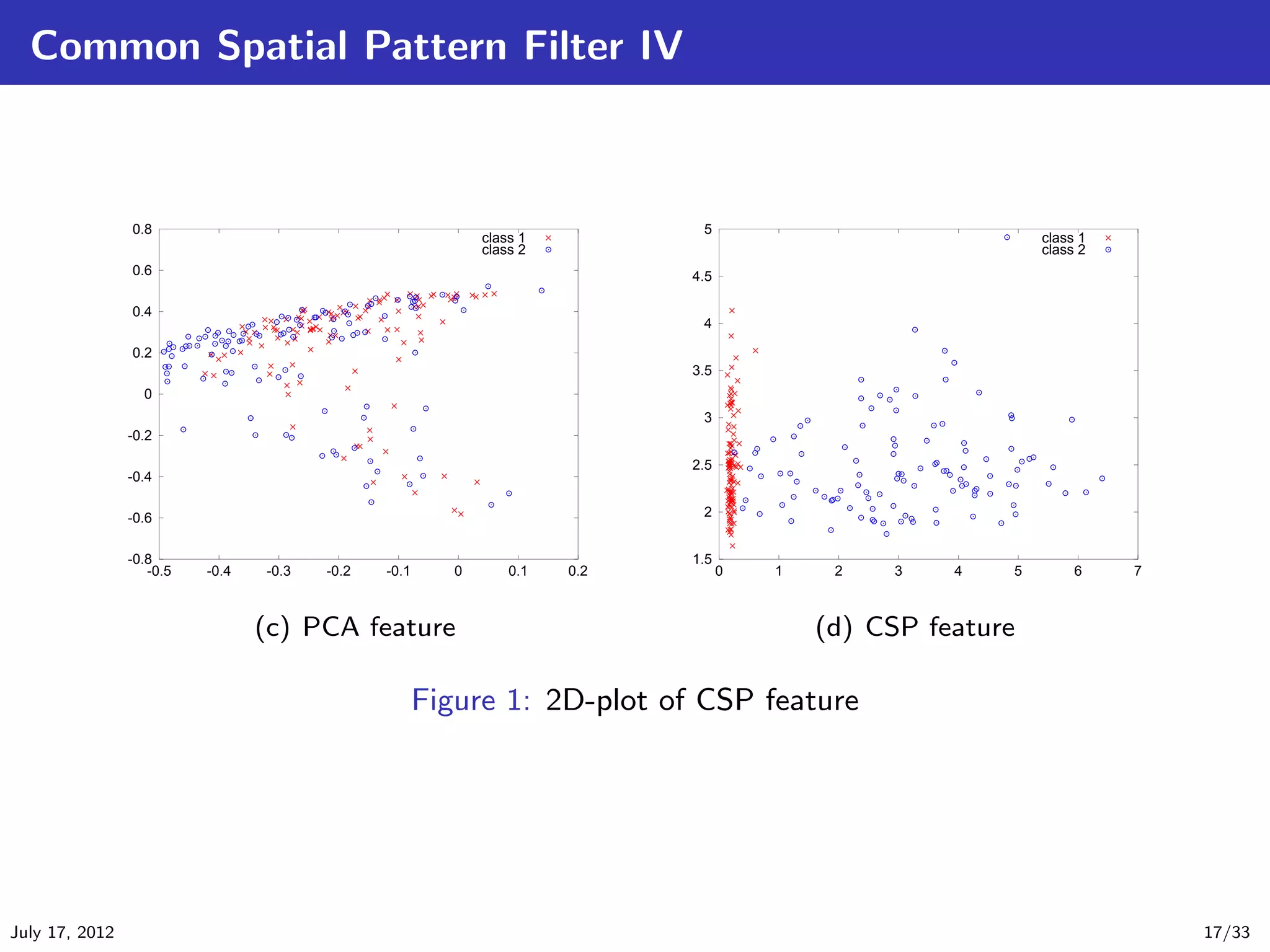
![Common Spatial Pattern Filter I
In previous example, we do not use a spatial filter. The proper spatial filter would provide signals
so that easy to classify. The goal of this study is to design spatial filters that lead to optimal
variances for the discrimination of two populations of EEG related to right hand and right foot
motor imagery. We call this method the “Common Spatial Pattern” (CSP) algorithm
[Muller-Gerking et al., 1999].
We denote the CSP filter by
S = W T E or s(t) = W T e(t), (12)
where W ∈ Rd×ch is spatial filter matrix, S ∈ Rd×time is filtered signal matrix.
The criterion of CSP is given by
maximize trW T Σ1 W , (13)
subject to W T (Σ1 + Σ2 )W = I, (14)
where
En EnT
Σ1 = Exp T
, (15)
En ∈{class 1} trEn En
En EnT
Σ2 = Exp T
. (16)
En ∈{class 2} trEn En
This problem can be solved by generalized eigen value problem. However, we can also solve it
by two times of standard eigen value problem.
July 17, 2012 14/33](https://image.slidesharecdn.com/main-120718022005-phpapp01/75/Introduction-to-Common-Spatial-Pattern-Filters-for-EEG-Motor-Imagery-Classification-14-2048.jpg)
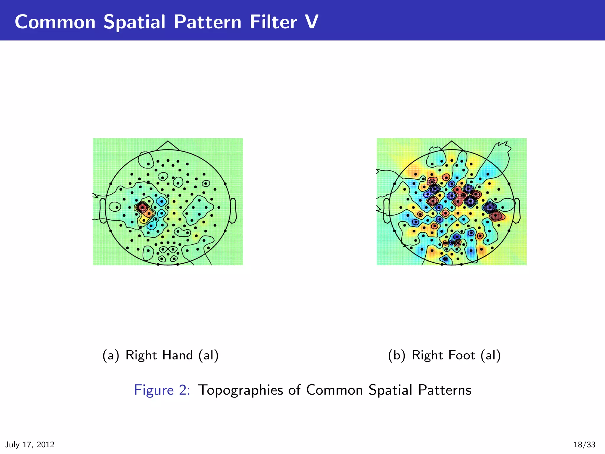
![Common Spatial Pattern Filter III
We have
λ1
T ..
W Σ1 W = Λ = . , (22)
λch
1 − λ1
..
W T Σ2 W = I − Λ = . , (23)
1 − λch
where λ1 ≥ λ2 ≥ · · · ≥ λch . Therefore, first CSP filter w1 provides maximum variance of class
1, and last CSP filter wch provides maximum variance of class 2.
We select first and last m filters to use as
Wcsp = w1 ··· wm wch−m+1 ··· wch ∈ R2m×ch , (24)
and filtered signal matrix is given by
T
T
s(t) = Wcsp e(t) = s1 (t) ··· sd (t) , (25)
i.e., d = 2m.
Feature vector x = (x1 , x2 , . . . , xd )T is calculated by
var[si (t)]
xi = log d
. (26)
i=1 var[si (t)]
July 17, 2012 16/33](https://image.slidesharecdn.com/main-120718022005-phpapp01/75/Introduction-to-Common-Spatial-Pattern-Filters-for-EEG-Motor-Imagery-Classification-16-2048.jpg)
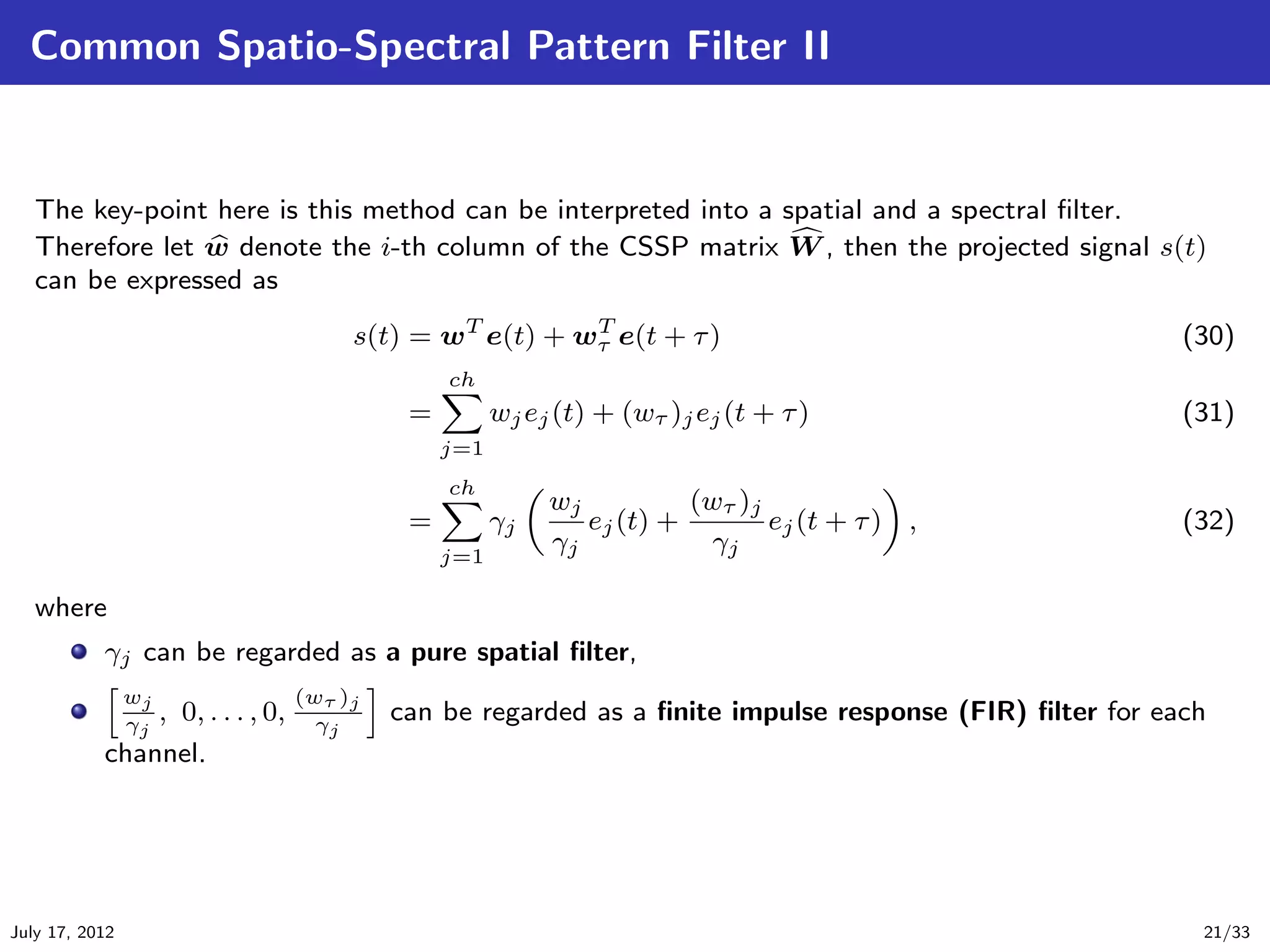
![Common Spatio-Spectral Pattern Filter I
The Common Spatio-Spectral Pattern (CSSP) filter is an extension of the CSP filter
[Lemm et al., 2005]. The CSSP can be regarded as a CSP method with the time delay
embedding.
The algorithm is not so different from the standard CSP. In CSP, we consider the following
transformation
S = W T E or s(t) = W T e(t). (27)
But the CSSP’s transform is given by
E
S = W T E + Wτ Eτ = W T
T
, (28)
Eτ
e(t)
or s(t) = W T e(t) + Wτ e(t + τ ) = W T
T
, (29)
e(t + τ )
where Eτ is a τ -time delayed signal matrix of E, and W T = [W T , Wτ ] is a CSSP matrix. It
T
can be also regarded that the number of channels increase to double. The deference between
CSP and CSSP is only this point, and then we can apply this method easily in a same way to the
CSP algorithm. However, τ is a hyper-parameter.
July 17, 2012 20/33](https://image.slidesharecdn.com/main-120718022005-phpapp01/75/Introduction-to-Common-Spatial-Pattern-Filters-for-EEG-Motor-Imagery-Classification-20-2048.jpg)
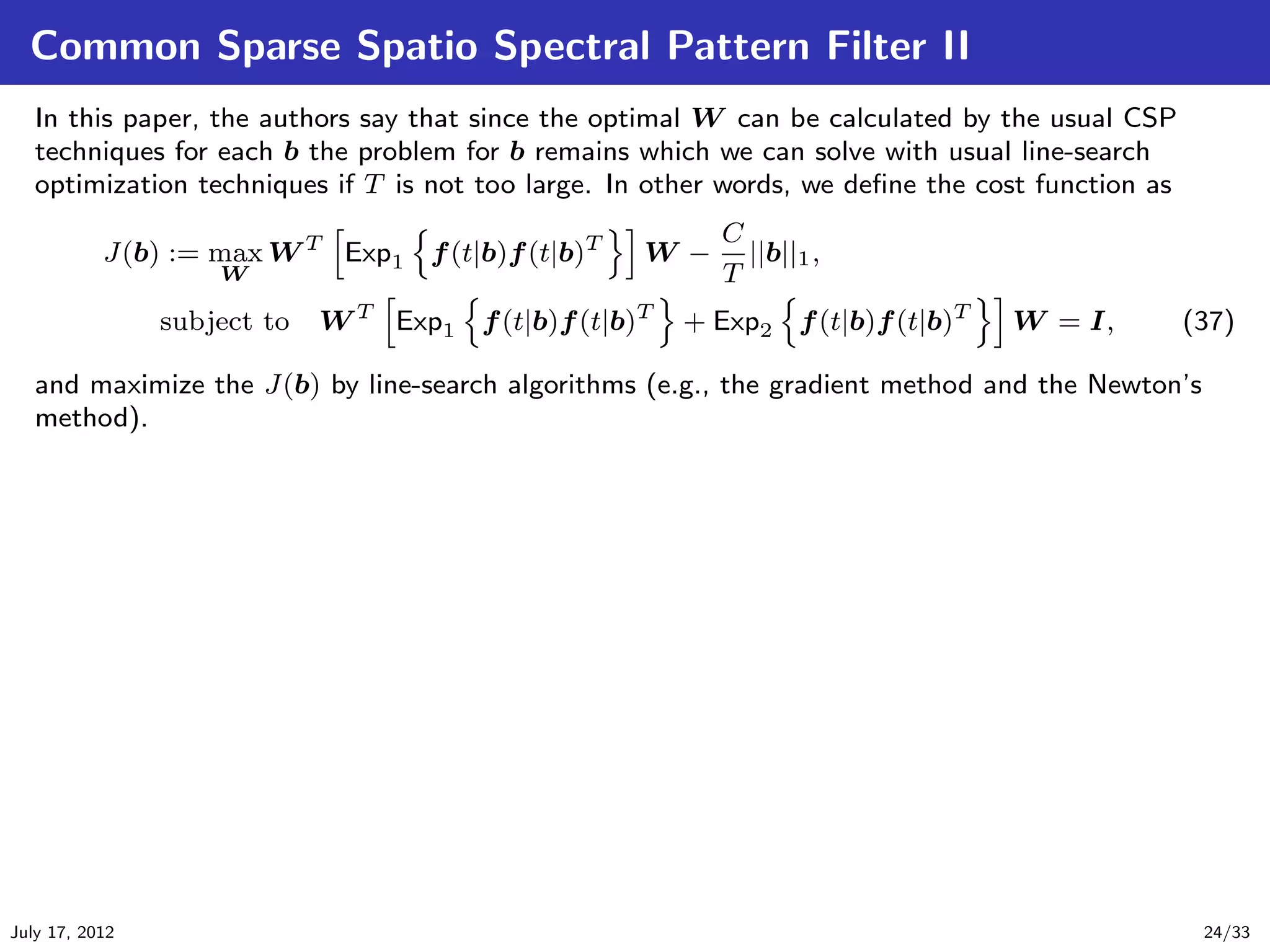
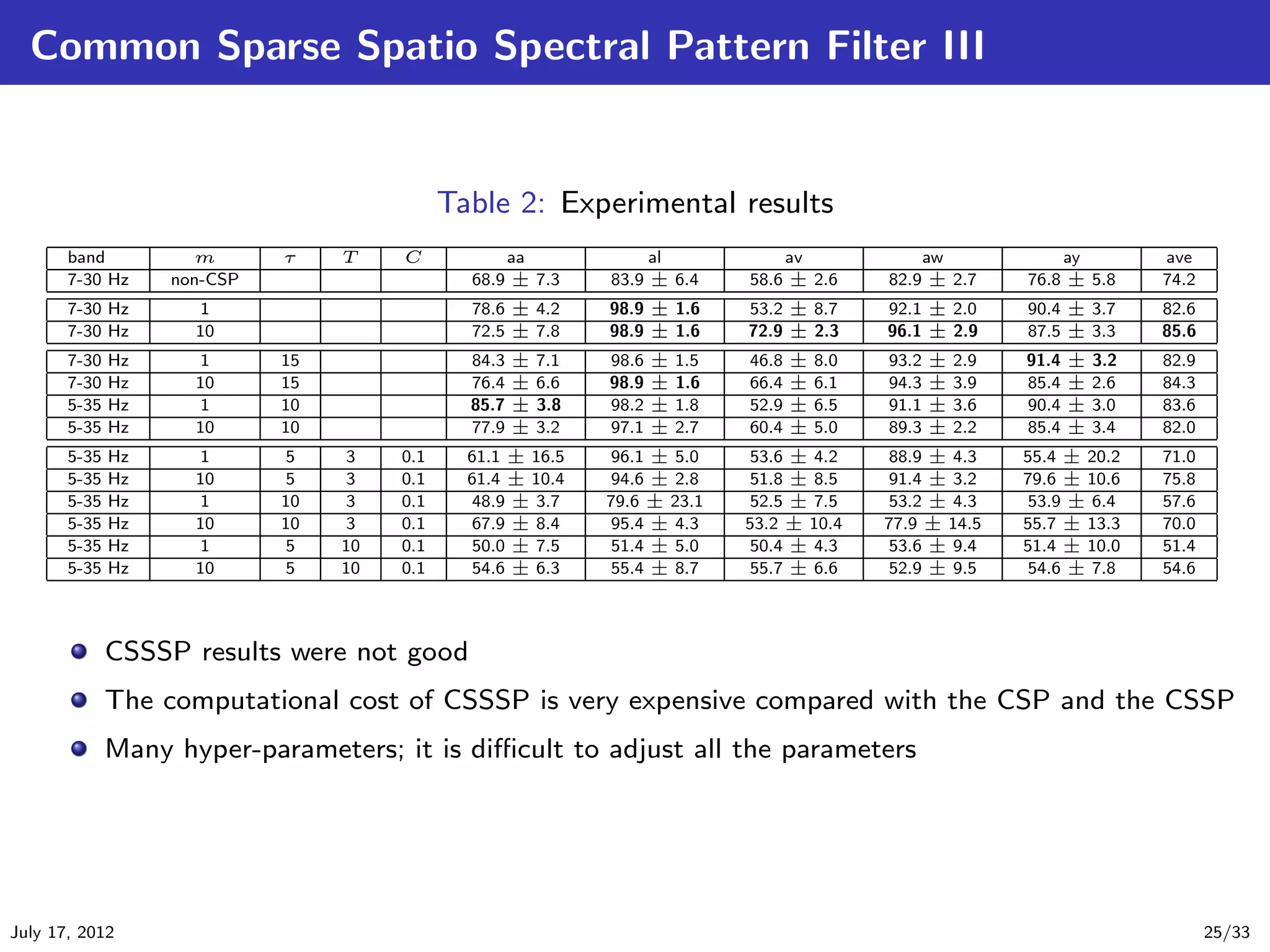
![Common Sparse Spatio Spectral Pattern Filter I
The Common Sparse Spatio Spectral Pattern (CSSSP) filter is a further extension of the CSSP
[Dornhege et al., 2005]. In CSSP’s FIR filter consists of only one time delay. The CSSSP’s FIR
filter is given by
f (t|b) = b0 e(t) + b1 e(t + τ ) + b2 + e(t + 2τ ) + · · · + bT e(t + T τ ) (33)
so that b is sparse spectral filter. Therefore, final signals are given by
T
s(t) = W T f (t|b) = bk W T e(t + kτ ). (34)
k=0
The criterion of CSSSP is given by
C
max max W T Exp1 f (t|b)f (t|b)T W − ||b||1 , (35)
b W T
subject to W T Exp1 f (t|b)f (t|b)T + Exp2 f (t|b)f (t|b)T W =I (36)
where
Exp1 {·} and Exp2 {·} denote the expectations for samples of class 1 and class 2,
respectively.
July 17, 2012 23/33](https://image.slidesharecdn.com/main-120718022005-phpapp01/75/Introduction-to-Common-Spatial-Pattern-Filters-for-EEG-Motor-Imagery-Classification-23-2048.jpg)
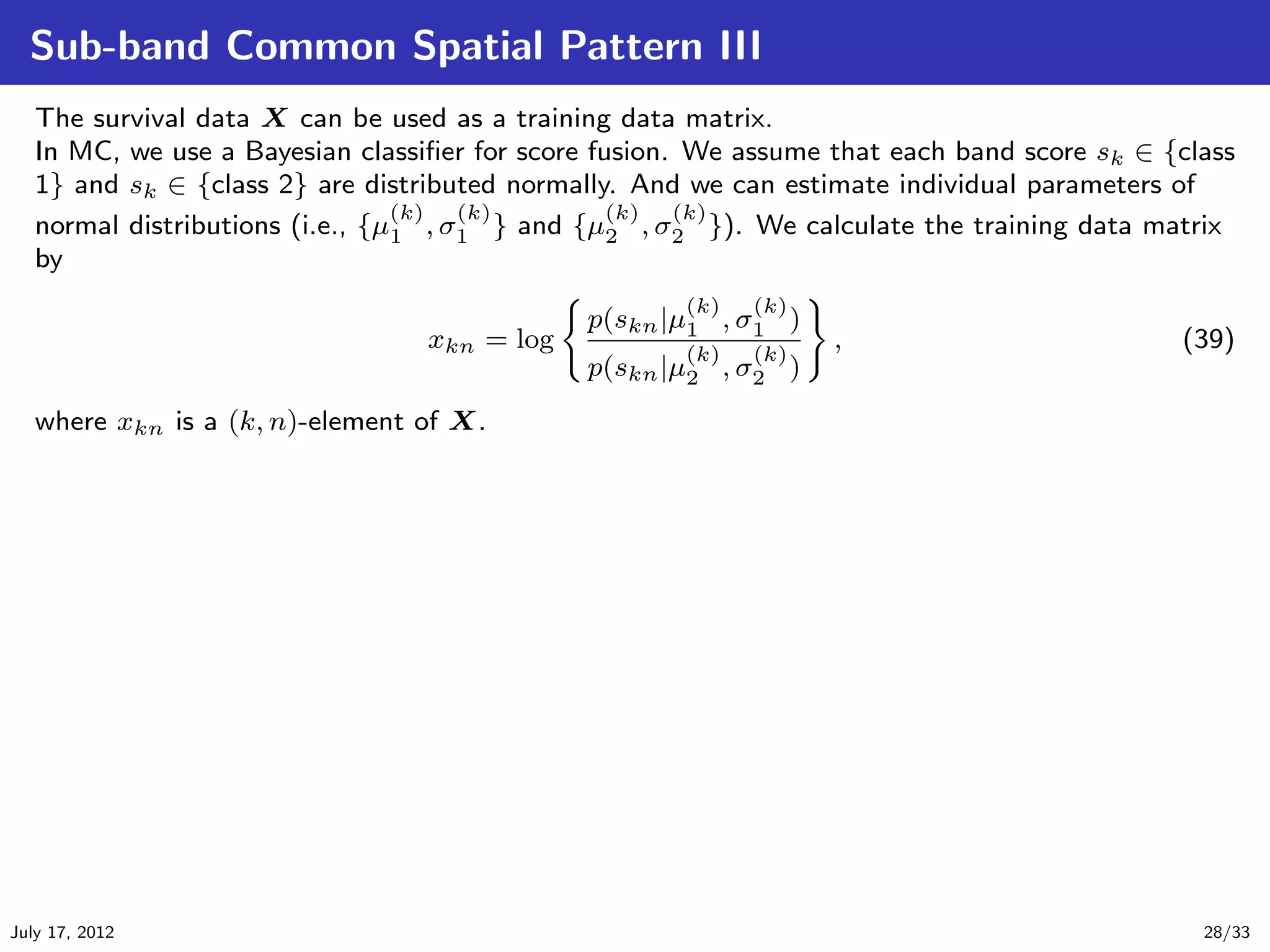
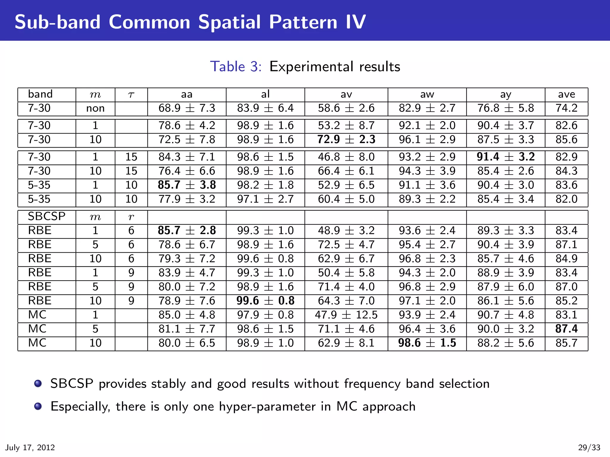
![Sub-band Common Spatial Pattern I
The CSP, the CSSP need the selection of frequency band to use band-pass filter at first
The CSSSP solutions are depend greatly on the initial points
Here, we introduce an alternative method based on Sub-band CSP (SBCSP) method and score
fusion [Novi et al., 2007].
Figure 3: System Flowchart of SBCSP: for example frequency bands of individual filters
are 4-8Hz, 8-12Hz, ... , 36-40Hz.
The processes until CSP filters are the same as it is. And then we obtain individual CSP feature
data matrices {F (1) , F (2) , . . . , F (K) }. The process of LDA score is given by follow:
July 17, 2012 26/33](https://image.slidesharecdn.com/main-120718022005-phpapp01/75/Introduction-to-Common-Spatial-Pattern-Filters-for-EEG-Motor-Imagery-Classification-26-2048.jpg)
![Sub-band Common Spatial Pattern II
Calculate the LDA projection vector w(k) for each data matrices F (k) .
LDA score vector is given by
(1)
w(1)T fn
w(2)T f (2)
n
sn =
. .
(38)
.
.
(K)
w(K)T fn
There are two approaches of score fusion method.
Recursive Band Elimination (RBE)
Meta-Classifier (MC)
In RBE, first we set a RBE-order that is a integer number r ∈ [1, K]. The first data set is
X = [s1 , ..., sN ] ∈ RK×N . In this method, we remove K − r rows from X by SVM feature
selection. The algorithm is follow
.
1 Train w by SVM
. Remove the row of X with the smallest w2
2
k
.
3 If number of rows of X is r algorithm is finished, else back to 1.
July 17, 2012 27/33](https://image.slidesharecdn.com/main-120718022005-phpapp01/75/Introduction-to-Common-Spatial-Pattern-Filters-for-EEG-Motor-Imagery-Classification-27-2048.jpg)
![Bibliography I
[Blankertz et al., 2006] Blankertz, B., Muller, K.-R., Krusienski, D., Schalk, G., Wolpaw, J. R.,
Schlogl, A., Pfurtscheller, G., del R. Millan, J., Schr¨der, M., and Birbaumer, N. (2006).
o
The bci competition iii: Validating alternative approaches to actual bci problems.
IEEE Trans. Neural Systems and Rihabilitation Engineering, 14:153–159.
[Dornhege et al., 2005] Dornhege, G., Blankertz, B., Krauledat, M., Losch, F., Curio, G., and
robert Muller, K. (2005).
Optimizing spatio-temporal filters for improving brain-computer interfacing.
In in Advances in Neural Inf. Proc. Systems (NIPS 05, pages 315–322. MIT Press.
[Hema et al., 2009] Hema, C., Paulraj, M., Yaacob, S., Adom, A., and Nagarajan, R. (2009).
Eeg motor imagery classification of hand movements for a brain machine interface.
Biomedical Soft Computing and Human Sciences, 14(2):49–56.
[Lemm et al., 2005] Lemm, S., Blankertz, B., Curio, G., and Muller, K.-R. (2005).
Spatio-spectral filters for improving the classification of single trial eeg.
Biomedical Engineering, IEEE Transactions on, 52(9):1541 –1548.
[Minka et al., 1999] Minka, S., Ratsch, G., Weston, J., Scholkopf, B., and Mullers, K. (1999).
Fisher discriminant analysis with kernels.
In Neural Networks for Signal Processing IX, 1999. Proceedings of the 1999 IEEE Signal
Processing Society Workshop, pages 41 –48.
July 17, 2012 31/33](https://image.slidesharecdn.com/main-120718022005-phpapp01/75/Introduction-to-Common-Spatial-Pattern-Filters-for-EEG-Motor-Imagery-Classification-31-2048.jpg)
![Bibliography II
[Muller-Gerking et al., 1999] Muller-Gerking, J., Pfurtscheller, G., and Flyvbjerg, H. (1999).
Designing optimal spatial filters for single-trial eeg classification in a movement task.
Clinical Neurophysiology, 110(5):787 – 798.
[Novi et al., 2007] Novi, Q., Guan, C., Dat, T. H., and Xue, P. (2007).
Sub-band common spatial pattern (sbcsp) for brain-computer interface.
In Neural Engineering, 2007. CNE ’07. 3rd International IEEE/EMBS Conference on, pages
204 –207.
July 17, 2012 32/33](https://image.slidesharecdn.com/main-120718022005-phpapp01/75/Introduction-to-Common-Spatial-Pattern-Filters-for-EEG-Motor-Imagery-Classification-32-2048.jpg)


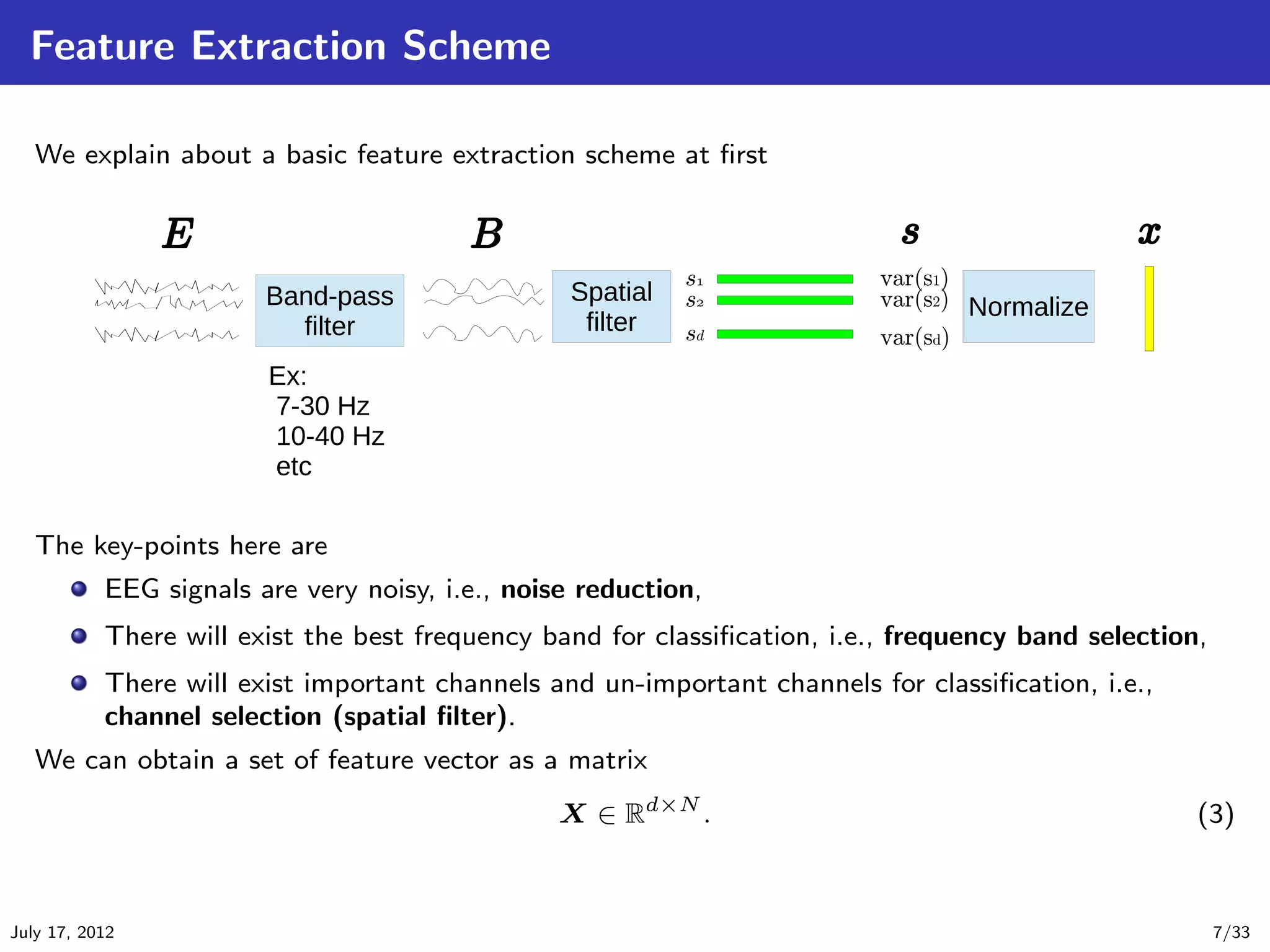
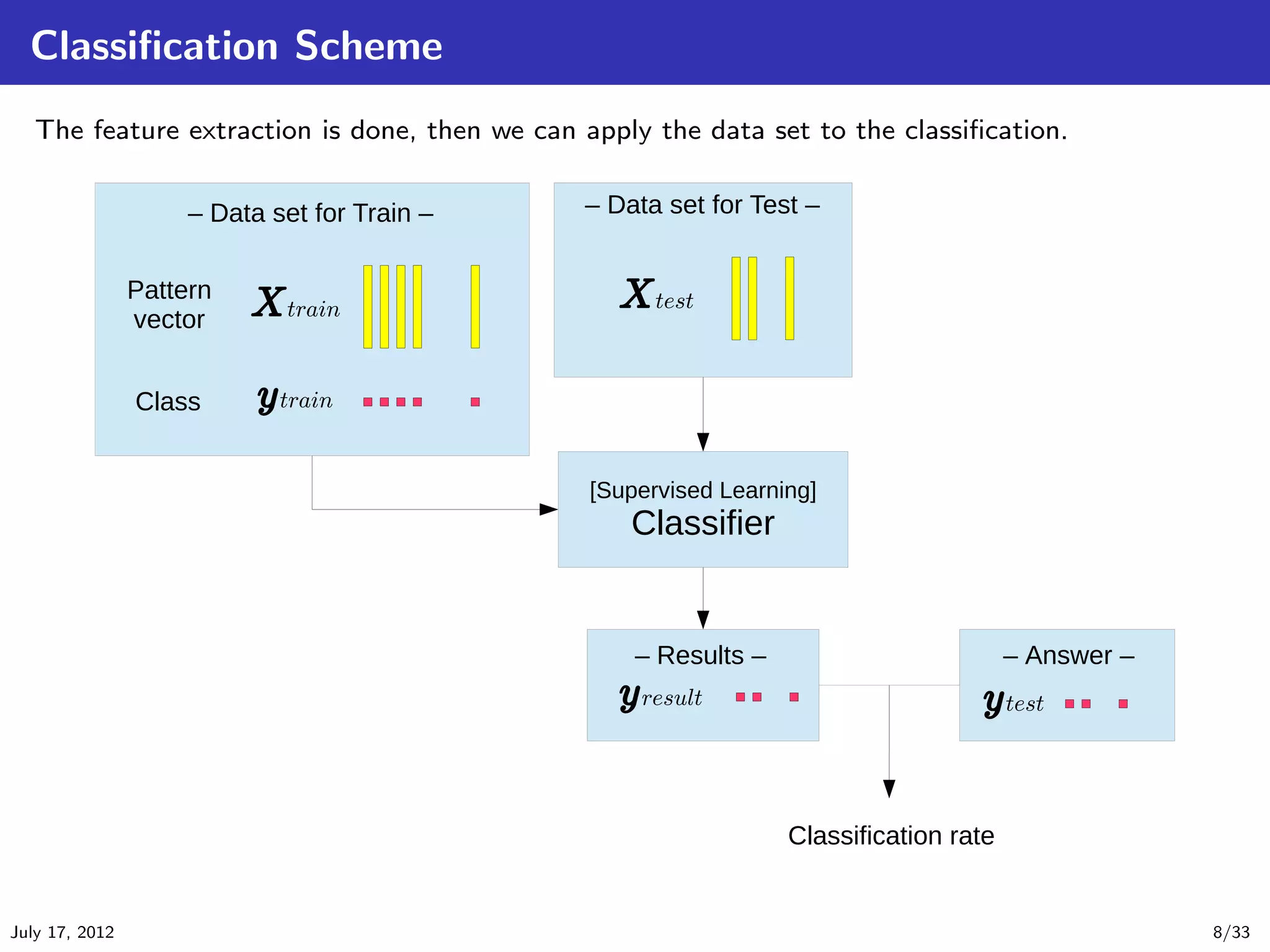
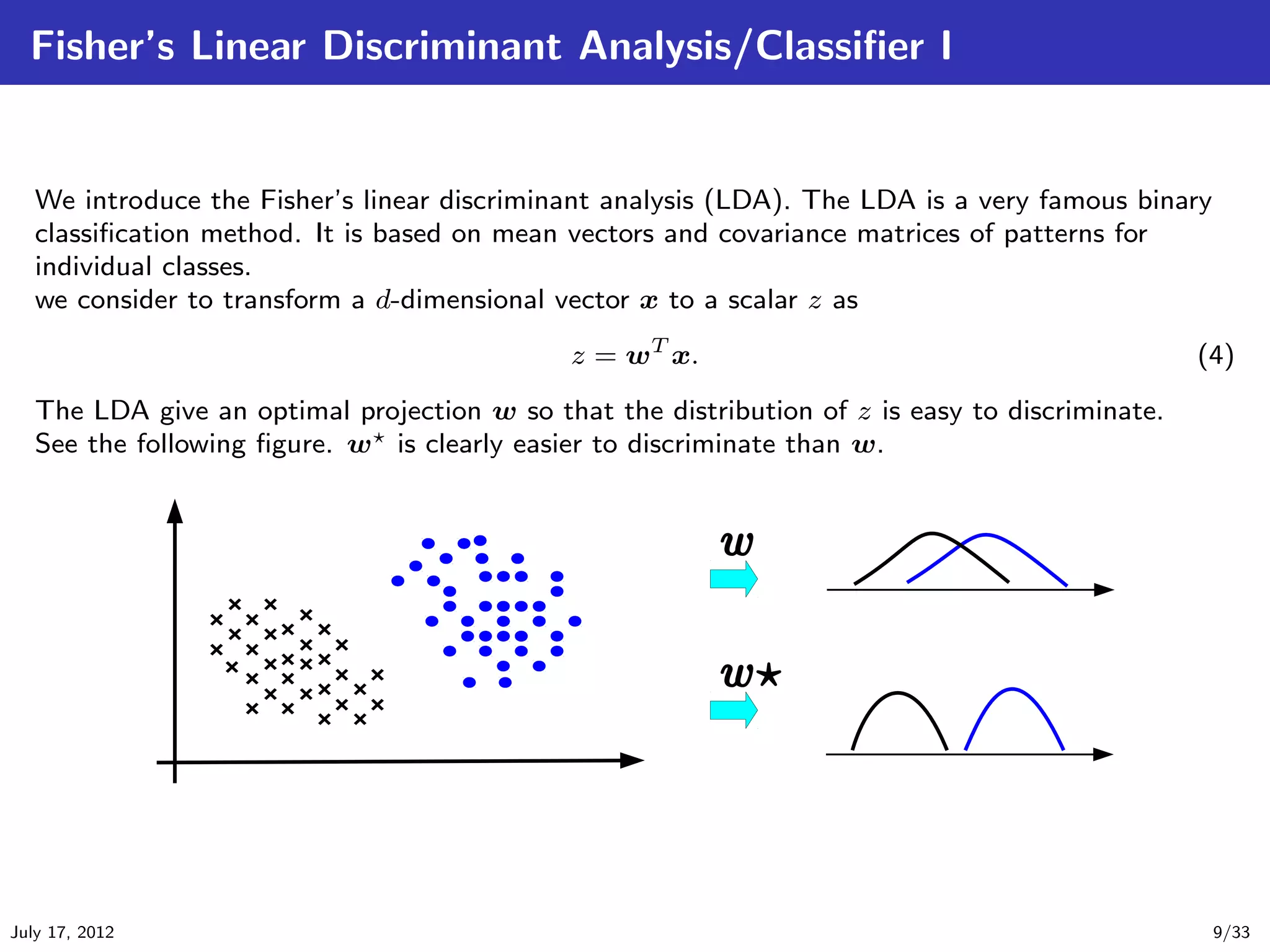
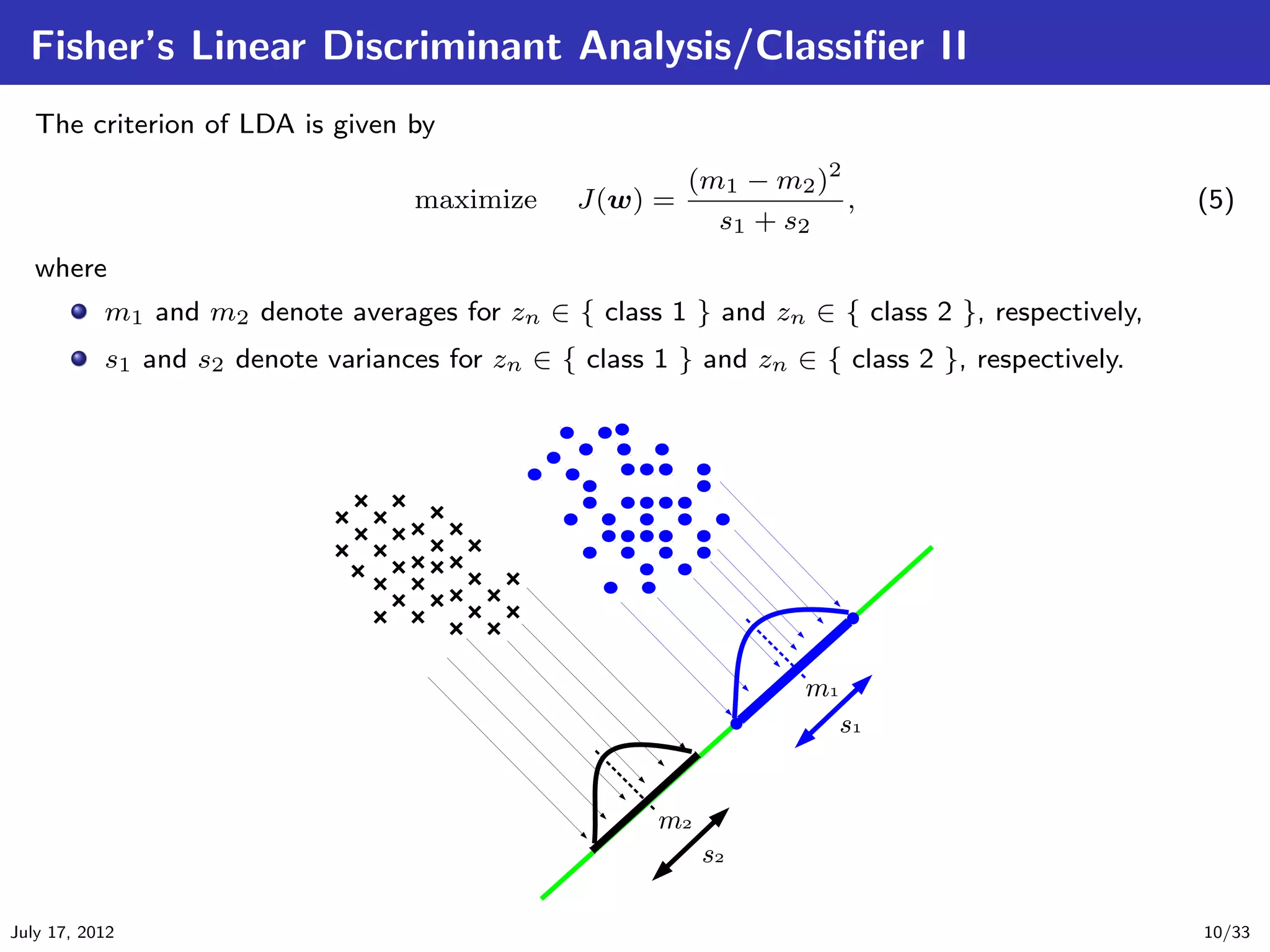
This document introduces common spatial pattern (CSP) filters for EEG motor imagery classification. CSP filters aim to find spatial patterns in EEG data that maximize the difference between two classes. The document outlines several CSP algorithms including standard CSP, common spatially standardized CSP, and spatially constrained CSP. CSP filters extract discriminative features from EEG data that can improve classification accuracy for brain-computer interface applications involving motor imagery tasks.


![Coded Agents – with UiPath SDK + LangGraph [Virtual Hands-on Workshop]](https://cdn.slidesharecdn.com/ss_thumbnails/codedagentsdeck-251215155422-5497c599-thumbnail.jpg?width=640&height=640&fit=bounds)