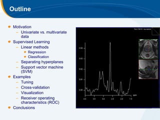
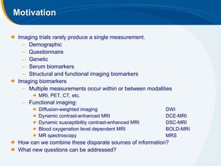
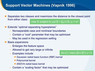
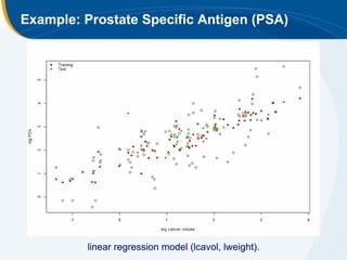
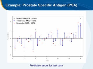
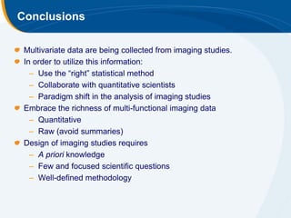
The document discusses the application of statistical techniques in multi-functional imaging trials, emphasizing the importance of multivariate data analysis over univariate methods. It covers various supervised learning methods, particularly focusing on support vector machines (SVM) for classification of imaging data, and includes examples from breast and prostate cancer studies. Conclusions highlight the need for appropriate statistical methods and collaboration with quantitative scientists to harness the full potential of imaging data.

1. Statistical Techniques for
Multi-functional Imaging Trials
Brandon Whitcher, PhD
Image Analysis & Mathematical Biology
Clinical Imaging Centre, GlaxoSmithKline

2. Declaration of Conflict of Interest or
Relationship
Speaker Name: Brandon Whitcher
I have the following conflict of interest to disclose with regard to
the subject matter of this presentation:
Company name: GlaxoSmithKline
Type of relationship: Employment

3. Outline
Motivation
– Univariate vs. multivariate
data
Supervised Learning
– Linear methods
Regression
Classification
– Separating hyperplanes
– Support vector machine
(SVM)
Examples
– Tuning
– Cross-validation
– Visualization
– Receiver operating
characteristics (ROC)
Conclusions

4. Motivation
Imaging trials rarely produce a single measurement.
– Demographic
– Questionnaire
– Genetic
– Serum biomarkers
– Structural and functional imaging biomarkers
Imaging biomarkers
– Multiple measurements occur within or between modalities
MRI, PET, CT, etc.
– Functional imaging:
Diffusion-weighted imaging DWI
Dynamic contrast-enhanced MRI DCE-MRI
Dynamic susceptibility contrast-enhanced MRI DSC-MRI
Blood oxygenation level dependent MRI BOLD-MRI
MR spectroscopy MRS
How can we combine these disparate sources of information?
What new questions can be addressed?

5. Neuroscience Example
Fig. 1. Voxel-based-morphometry (VBM) analysis showing an additive effect of the APOE ε4
allele (APOE4) on grey matter volume (GMV).
Filippini et al. NeuroImage 2008

6. Motivation (cont.)
Univariate statistical methods
– One method → one measurement → answer one question
– One method → multiple measurements
Measurement #1 → answer question #1
Measurement #2 → answer question #1
…
Multivariate statistical methods
– Method #1 → one measurement
– Method #2 → multiple measurements answer one question
– Method #3 → multiple measurements
– …
Goal = Prediction (e.g., computer-aided diagnosis)
– Supervised learning procedures

7. What is Supervised Learning?
T1, T2, DWI, Regression,
DCE-MRI, LDA, SVM,
MRS, Genetics
Test Data
NN
Step 2
Training Supervised
Model
Data Learning
Step 1
Benign, Results
malignant

8. Linear Regression
Given a set of inputs X = (X1, X2, …, Xp), want to predict Y
– Linear regression model: f(X) = β0 + ∑j Xjβj
– Minimize residual sum of squares: RSS(β) = ∑i (yi – f(xi))2

9. Linear Methods for Classification
Linear Discriminant Analysis (LDA)
– Procedure:
Estimate mean vectors and covariance matrix
Calculate linear decision boundaries
Classify points using linear decision boundaries
Logistic regression is another popular method
– Binary outcome with qualitative/quantitative predictors
– Maximize likelihood via iteratively re-weighted least squares
Neither method was designed to explicitly separate data.
– LDA = optimized when mean vector and covariance is known
– Logistic regression = to understand the role of the input variables

10. LDA w/ Two Classes: Step-by-Step
Measurement #2
Measurement #1

11. LDA w/ Three Classes: Step-by-Step
Measuring #2
Measurement #1

12. Separating Hyperplanes
Rosenblatt’s Perceptron Learning Algorithm (1958)
– Minimizes the distance of misclassified points to the decision
boundary:
min D(β,β0) = –∑iєM yi(xTβ + β0); yi = ±1
– Converges in a “finite” number of steps.
Problems (Ripley, 1996)
1. Separable data implies many solutions (initial conditions).
2. Slow convergence... smaller the gap = longer the time.
3. Nonseparable data implies the algorithm will not converge!
Optimal separating hyperplanes (Vapnik and Chervonenkis, 1963)
– Forms the foundation for support vector machines.

13. Separating Hyperplanes: separable case
optimal

14. Support Vector Machines (Vapnik 1996)
Separates two classes and maximizes the distance to the closest point
from either class:
max C subject to yi(xTβ + β0) ≥ C; yi = ±1
Extends “optimal separating hyperplanes”
– Nonseparable case and nonlinear boundaries
– Contain a “cost” parameter that may be optimized
– May be used in the regression setting
Basis expansions
– Enlarges the feature space
– Allowed to get very large or infinite
– Examples include k(x,x′) = exp(-γ║x-x′║2); γ > 0
Gaussian radial basis function (RBF) kernel
Polynomial kernel
ANOVA radial basis kernel
– Contain a “scaling factor” that may be optimized

15. Support Vector Classifiers: separable case
1
C

1 margin
C

support point
Adapted from Hastie, Tibshirani and Friedman (2001)
xT   0  0

16. Support Vector Classifiers: nonseparable case
1
C

1 margin
C

4

5

 1
3

2

Adapted from Hastie, Tibshirani and Friedman (2001)
xT   0  0

17. Support Vector Machine: Spiral Example

18. Support Vector Machine: Spiral Example

19. Receiver Operating Characteristic (ROC)
Graphical plot of sensitivity vs. (1 – specificity)
– Binary classifier system as discrimination threshold varies
actual value
p n total 2×2 contingency table
True False
p’ Positive Positive P’
prediction
outcome False True
n’ Negative Negative N’
total P N
Sensitivity = True Positive Rate = TP / (TP + FN)
Specificity = 1 – False Positive Rate = 1 – FP / (FP + TN)

20. Example: Breast Cytology
699 samples
– 9 measurements (ordinal)
Clump thickness
Cell size uniformity
Cell shape uniformity
Marginal adhesion
Single epithelial cell size
Bare nuclei
Bland chromatin
Normal nucleoli
Mitoses
– 2 classes
Benign
Malignant
Classification problem since
outcome measure is binary.
Train = 550, Test = 133.
Wolberg & Mangasarian (1990)

21. Example: Breast Cytology

22. Example: Breast Cytology
Diagnostic plot from SVM procedure.

23. Example: Breast Cytology
Response surface to SVM parameters.

24. Example: Breast Cytology
Logistic Regression
Benign Malignant
Benign 84 5
sensitivity = 95.5%
Malignant 4 40 specificity = 88.9%
Linear Discriminant Analysis
Benign Malignant
Benign 90 6
sensitivity = 98.9%
Malignant 1 36
specificity = 85.7%
Naïve Support Vector Machine
Benign Malignant
Benign 89 2
sensitivity = 97.8%
specificity = 95.2%
Malignant 2 40
Tuned Support Vector Machine
Benign Malignant
sensitivity = 97.8%
Benign 89 1
specificity = 97.6%
Malignant 2 41

25. Example: Breast Cytology
Sensitivity
1 - Specificity
Receiver operating characteristic (ROC) plot.

26. Example: Prostate Specific Antigen (PSA)
Stamey et al. (1989); used in Hastie, Tibshirani and Friedman (2001).
Correlation between the level of PSA and various clinical measures (N = 97)
– log cancer volume,
– log prostate weight,
– log of BPH amount,
– seminal vesicle invasion,
– log of capsular penetration,
– Gleason score, and
– percent of Gleason scores 4 or 5.
Regression problem since outcome measure is quantitative.
Training data = 67, Test data = 30.

27. Example: Prostate Specific Antigen (PSA)

28. Example: Prostate Specific Antigen (PSA)
Best subset selection for linear regression model.

29. Example: Prostate Specific Antigen (PSA)
linear regression model (lcavol, lweight).

30. Example: Prostate Specific Antigen (PSA)
Response surface to SVM parameters.

31. Example: Prostate Specific Antigen (PSA)
Prediction errors for test data.

32. Conclusions
Multivariate data are being collected from imaging studies.
In order to utilize this information:
– Use the “right” statistical method
– Collaborate with quantitative scientists
– Paradigm shift in the analysis of imaging studies
Embrace the richness of multi-functional imaging data
– Quantitative
– Raw (avoid summaries)
Design of imaging studies requires
– A priori knowledge
– Few and focused scientific questions
– Well-defined methodology

33. Acknowledgments
Anwar Padhani
Roberto Alonzi
Claire Allen
Mark Emberton
Henkjan Huisman
Giulio Gambarota

34. Bibliography
Filippini N, Rao, A, et al. Anatomically-distinct genetic associations of APOE ε4 allele
load with regional cortical atrophy in Alzheimer's disease. NeuroImage 2009, 44:724-
728.
Freer TW, Ulissey, MJ. Screening Mammography with Computer-aided Detection:
Prospective Study of 12,860 Patients in a Community Breast Center. Radiology 2001,
220:781-786.
Hastie T, Tibshirani, R, Freidman, J. The Elements of Statistical Learning, Springer,
2001.
McDonough KL. Breast Cancer Stage Cost Analysis in a Manage Care Population.
American Journal of Managed Care 1999, 5(6):S377-S382.
R Development Team. R: A Language and Environment for Statistical Computing. R
Foundation for Statistical Computing, Vienna, Austria.
– www.R-project.org
– R package e1071
– R package mlbench
Ripley, BD. Pattern Recognition and Neural Networks, Cambridge University Press,
1996.
Vos PC, Hambrock, T, et al. Computerized analysis of prostate lesions in the peripheral
zone using dynamic contrast enhanced MRI. Medical Physics 2008, 35(3):888-899.
Wolberg WH, Mangasarian, OL. Multisurface method of pattern separation for medical
diagnosis applied to breast cytology. PNAS 1990, 87(23):9193-9196.