Svm

SVMs

• Geometric
– Maximizing Margin
• Kernel Methods
– Making nonlinear decision boundaries linear
– Efficiently!
• Capacity
– Structural Risk Minimization

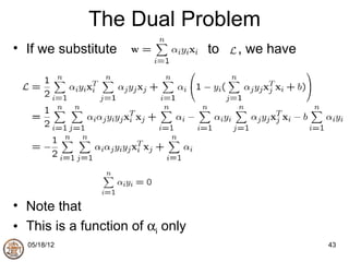
SVM History
• SVM is a classifier derived from statistical learning
theory by Vapnik and Chervonenkis
• SVM was first introduced by Boser, Guyon and
Vapnik in COLT-92
• SVM became famous when, using pixel maps as
input, it gave accuracy comparable to NNs with
hand-designed features in a handwriting
recognition task
• SVM is closely related to:
– Kernel machines (a generalization of SVMs), large
margin classifiers, reproducing kernel Hilbert space,
Gaussian process, Boosting

α
Linear Classifiers
x f yest
f(x,w,b) = sign(w. x - b)
denotes +1
denotes -1

How would you
classify this data?

α
Linear Classifiers
x f yest
denotes +1
denotes -1

Any of these
would be fine..

..but which is
best?

α
Classifier Margin
x f yest
denotes +1
denotes -1 Define the margin
of a linear
classifier as the
width that the
boundary could be
increased by
before hitting a
datapoint.

α
Maximum Margin
x f yest
denotes +1
denotes -1 The maximum
margin linear
classifier is the
linear classifier
with the maximum
margin.
This is the
simplest kind of
SVM (Called an
LSVM)
Linear SVM

α
Maximum Margin
x f yest
denotes +1
margin linear
classifier is the
linear classifier
Support Vectors with the, um,
are those
datapoints that maximum margin.
the margin
This is the
pushes up
against simplest kind of
SVM (Called an
LSVM)
Linear SVM

Why Maximum Margin?
1. Intuitively this feels safest.
2. If we’ve made a small error in the
denotes +1
location of the boundary (it’s been
jolted in its perpendicular direction)
this gives us least chance linear
margin of causing a
misclassification. classifier is the
linear classifier
3. There’s some theory (using VC
Support Vectors dimension) that is related to um, not
with the, (but
are those the same as) the proposition that this
datapoints that maximum margin.
is a good thing.
the margin
This is the
4. Empirically it works very very well.
pushes up
against simplest kind of
SVM (Called an
LSVM)

A “Good” Separator

O O
X X
X O
X O O
X X O
X O
X O

Noise in the Observations

O O
X X
X O
X O O
X X O
X O
X O

Ruling Out Some Separators

O O
X X
X O
X O O
X X O
X O
X O

Lots of Noise

O O
X X
X O
X O O
X X O
X O
X O

Maximizing the Margin

O O
X X
X O
X O O
X X O
X O
X O

Specifying a line and margin

”
= +1 Plus-Plane
s
C las e Classifier Boundary
dict zon
“ Pre Minus-Plane
= -1”
s
C l as
dict zone
“ Pre

• How do we represent this mathematically?
• …in m input dimensions?

Specifying a line and margin
”
= +1 Plus-Plane
s
C las e Classifier Boundary
ict zon
“Pred Minus-Plane
= -1”
s
=1 C l as
wx
+b
=0 dict zone
+ b -1
w x b= “ Pre
+
wx

• Plus-plane = { x : w . x + b = +1 }
• Minus-plane = { x : w . x + b = -1 }
Classify +1 if w . x + b >= 1
as..
-1 if w . x + b <= -1
Universe if -1 < w . x + b < 1
explodes

Computing the margin width
”
= +1 M = Margin Width
s
C las e
ict zon
“Pred
= -1” How do we compute
s
=1 C l as M in terms of w
wx
+b
=0 dict zone
+ b -1
w x b= “ Pre and b?
+
wx

• Plus-plane = { x : w . x + b = +1 }
• Minus-plane = { x : w . x + b = -1 }
Claim: The vector w is perpendicular to the Plus
Plane. Why?

”
s
C las e
ict zon
“Pred
= -1” How do we compute
s
=1 C l as M in terms of w
wx
+b
=0 dict zone
+ b -1
w x b= “ Pre and b?
+
wx

• Plus-plane = { x : w . x + b = +1 }
• Minus-plane = { x : w . x + b = -1 }
Claim: The vector w is perpendicular to the Plus
Plane. Why? Let u and v be two vectors on the
Plus Plane. What is w . ( u – v ) ?

And so of course the vector w is also
perpendicular to the Minus Plane

”
s x+
C las e
ict zon
“Pred
=- -
1” How do we compute
x
=1 l as s M in terms of w
+b i ct C zone
wx =0
+ b -1 “Pred and b?
w x b=
+
wx

• Plus-plane = { x : w . x + b = +1 }
• Minus-plane = { x : w . x + b = -1 }
• The vector w is perpendicular to the Plus Plane in
Any location
R : not
A : not m
m

• Let x- be any point on the minus plane necessarily a
datapoint
• Let x+ be the closest plus-plane-point to x-.

”
s x+
C las e
ict zon
“Pred
=- -
x
=1 l as s M in terms of w
+b i ct C zone
wx =0
+ b -1 “Pred and b?
w x b=
+
wx

• Plus-plane = { x : w . x + b = +1 }
• Minus-plane = { x : w . x + b = -1 }
• The vector w is perpendicular to the Plus Plane
• Let x- be any point on the minus plane
• Claim: x+ = x- + λ w for some value of λ. Why?

”
s x+
C las e
ict zon The line from x- to x+ is
“Pred
--
perpendicular to the
=
ss x planes.terms of w
M in
b=
1 Cla e
ct zon
+ i
wx =0
+ b -1 “Pred So to getbfrom x- to x+
and ?
w x b=
+
wx travel some distance in
• Plus-plane = { x : w . x + b =direction w.
+1 }
• Minus-plane = { x : w . x + b = -1 }
• The vector w is perpendicular to the Plus Plane
• Let x- be any point on the minus plane
• Claim: x+ = x- + λ w for some value of λ. Why?

”
s x+
C las e
ict zon
“Pred
1”
x =- -
=1 l as s
+b i ct C zone
wx =0
+ b -1 “Pred
w x b=
+
wx

What we know:
• w . x+ + b = +1
• w . x- + b = -1
• x+ = x- + λ w
• |x+ - x- | = M
It’s now easy to get M in terms of w and b

”
s x+
C las e
ict zon
“Pred
1”
x =- -
=1 l as s
+b i ct C zone
wx =0
+ b -1 “Pred w . (x - + λ w) + b = 1
w x b=
+
wx
=>

What we know: w . x + b + λ w .w = 1 -

• w . x+ + b = +1 =>
• w . x- + b = -1 -1 + λ w .w = 1
• x+ = x- + λ w => 2
λ=
• |x+ - x- | = M w.w
It’s now easy to get M in terms of w and b

” 2
= +1 M = Margin Width =
s x+
C las e w.w
ict zon
“Pred
1”
x =- -
=1 l as s
+b i ct C zone
wx =0
+ b -1 “Pred M= |x+ - x- | =| λ w |=
w x b=
+
wx

What we know: = λ | w | = λ w.w
• w . x+ + b = +1
2 w.w 2
• w . x- + b = -1 = =
w.w w.w
• x+ = x- + λ w
• |x+ - x- | = M
2
• λ=
w.w

Learning the Maximum Margin Classifier
” 2
= +1 M = Margin Width =
s x+
C las e w.w
ict zon
“Pred
1”
x =- -
=1 l as s
+b i ct C zone
wx =0
+ b -1 “Pred
w x b=
+
wx

Given a guess of w and b we can
• Compute whether all data points in the correct half-planes
• Compute the width of the margin
So now we just need to write a program to search the space
of w’s and b’s to find the widest margin that matches all the
datapoints. How?
Gradient descent? Simulated Annealing? Matrix Inversion?
EM? Newton’s Method?

Don’t worry…
it’s good for
you…
• Linear Programming

find w
argmax c⋅w
subject to
w⋅ai ≤ bi, for i = 1, …, m
wj ≥ 0 for j = 1, …, n
There are fast algorithms for solving linear programs including the
simplex algorithm and Karmarkar’s algorithm

Learning via Quadratic Programming

• QP is a well-studied class of optimization
algorithms to maximize a quadratic function
of some real-valued variables subject to
linear constraints.

Quadratic Programming
uT Ru
Find arg max c + dT u + Quadratic criterion
u 2

Subject to a11u1 + a12u 2 + ... + a1mum ≤ b1
a21u1 + a22u 2 + ... + a2 mu m ≤ b2 n additional linear
inequality
: constraints
an1u1 + an 2u 2 + ... + anmu m ≤ bn
And subject to

e additional linear
a( n +1)1u1 + a( n +1) 2u2 + ... + a( n +1) mu m = b( n +1)

constraints
equality
a( n + 2)1u1 + a( n + 2 ) 2u2 + ... + a( n + 2 ) mu m = b( n + 2 )
:
a( n + e )1u1 + a( n + e ) 2u2 + ... + a( n + e ) mu m = b( n + e )

Quadratic Programming
uT Ru
Find arg max c + dT u + Quadratic criterion
u 2

Subject to a11u1 + a12u 2 + ... + a1mum ≤ b1g
in
for find
re ex
u lg ... h e s qu m ≤ ic
a21u1 + a22ist2a+ orit+ md2 muadratb2
a n additional linear
Th e constra
in tl y
s uch : ore efficien inequality
much m n gradient constraints
optima a
lia...y th u ≤ b
bl
an1u1 + ann2d re+ ascennm m
a u2 + a t. n
ou
And subject to very f iddly…y e

e additional linear
are+ ... + a t to writ = b
a( n +1)1u1 (+ ut( nh1)y u2 n’t wan( n +1) mu m
B a t + e 2 do ( n +1)

constraints
equality
ly
probab yoursel
f)
a u +a
( n + 2 )1 1 uon+ ... + a
e
( n+ 2) 2 2 u =b
( n+ 2) m m ( n+2)

:
a( n + e )1u1 + a( n + e ) 2u2 + ... + a( n + e ) mu m = b( n + e )

Learning the Maximum Margin Classifier
” M=
= +1 2 Given guess of w , b we
s
C las e w.w can
dict zon
“ Pre • Compute whether all
= -1”
s
=1 C l as data points are in the
wx
+b
0 dict zone
+ b=
wx b=-1 “ Pre correct half-planes
+
wx
• Compute the margin
width
What should our How many constraints
Assume R datapoints,
quadratic optimization each (xhave? R yk =
will we k,yk) where
criterion be? What 1
+/- should they be?
Minimize w.w w . xk + b >= 1 if yk = 1
w . xk + b <= -1 if yk = -1

This is going to be a problem!
Uh-oh!
What should we do?
denotes +1 Idea 1:
denotes -1
Find minimum w.w, while
minimizing number of
training set errors.
Problem: Two things to
minimize makes for an
ill-defined optimization

Uh-oh!
What should we do?
denotes +1 Idea 1.1:
denotes -1
Minimize
w.w + C (#train errors)
Tradeoff parameter

There’s a serious practical
problem that’s about to make
us reject this approach. Can
you guess what it is?

Uh-oh!
What should we do?
denotes -1
Minimize
w.w + C (#train errors)
Tradeoff parameter
Can’t be expressed as a Quadratic
Programming problem.
Solving it may be too slow.
There’s a serious practical
(Also, doesn’t distinguish between
problem that’s abouteyr make
disastrous errors and near misses)
n
So… a to
o th
us reject this approach. Can
ideas?
you guess what it is?

Uh-oh!
What should we do?
denotes -1
Minimize
w.w + C (distance of error
points to their
correct place)

Learning Maximum Margin with Noise
M=
2 Given guess of w , b we
w.w can
• Compute sum of
b =1 distances of points to
w x+ 0
+ b=
wx b=-1
their correct zones
+
wx
width
What should our Assume R datapoints,
quadratic optimization each (xk,yk) where yk =
criterion be? +/- 1
How many constraints
will we have?
What should they be?

Large-margin Decision Boundary
• The decision boundary should be as far away from the data of both
classes as possible
– We should maximize the margin, m
– Distance between the origin and the line wtx=k is k/||w||

Class 2

m
Class 1

05/18/12 39

Finding the Decision Boundary
• Let {x1, ..., xn} be our data set and let yi ∈ {1,-1} be the
class label of xi
• The decision boundary should classify all points correctly ⇒

• The decision boundary can be found by solving the
following constrained optimization problem

• This is a constrained optimization problem. Solving it
requires some new tools
– Feel free to ignore the following several slides; what is important is
05/18/12 constrained optimization problem above
the 40

Back to the Original Problem

• The Lagrangian is

– Note that ||w||2 = wTw
• Setting the gradient of w.r.t. w and b to zero, we
have

05/18/12 41

• The Karush-Kuhn-Tucker conditions,

05/18/12 42

The Dual Problem
• If we substitute to , we have

• Note that
• This is a function of αi only
05/18/12 43

The Dual Problem
• The new objective function is in terms of αi only
• It is known as the dual problem: if we know w, we know all αi; if we
know all αi, we know w
• The original problem is known as the primal problem
• The objective function of the dual problem needs to be maximized!
• The dual problem is therefore:

Properties of αi when we introduce The result when we differentiate the
the Lagrange multipliers original Lagrangian w.r.t. b 44

The Dual Problem

• This is a quadratic programming (QP) problem
– A global maximum of αi can always be found

• w can be recovered by

05/18/12 45

Characteristics of the Solution
• Many of the αi are zero
– w is a linear combination of a small number of data points
– This “sparse” representation can be viewed as data compression
as in the construction of knn classifier
• xi with non-zero αi are called support vectors (SV)
– The decision boundary is determined only by the SV
– Let tj (j=1, ..., s) be the indices of the s support vectors. We can
write
• For testing with a new data z
– Compute and classify
z as class 1 if the sum is positive, and class 2 otherwise
– Note: w need not be formed explicitly

05/18/12 46

A Geometrical Interpretation
Class 2

α10=0
α8=0.6

α7=0
α2=0
α5=0

α1=0.8
α4=0
α6=1.4

α9=0
α3=0
Class 1

05/18/12 47

Non-linearly Separable Problems
• We allow “error” ξi in classification; it is based on the output of the
discriminant function wTx+b
• ξi approximates the number of misclassified samples

Class 2

Class 1
05/18/12 48

M=
ε11 2 Given guess of w , b we
ε2 w.w can
• Compute sum of
+b
=1 distances of points to
wx 0 ε7
+ b=
wx b=-1
their correct zones
+
wx
width
What should our How many R datapoints,
Assume constraints will
quadratic optimization we have?k,yk) where yk =
each (x R
criterion be? R What should they be?
+/- 1
1
Minimize w.w + C ∑ εk w . x + b >= 1-ε if y = 1
2 k =1
k k k

w . xk + b <= -1+εk if yk = -1

m = # input
M= dimensions
2 Given guess of w , b we
ε11
ε2 w.w can
• Compute sum m+1
Our original (noiseless data) QP had of
1 variables: w1, w2, … wm, and of points to
distances b.
b=
wx
+
0 ε7
Our new (noisy data) QP correct zones
their has m+1+R
+ b=
wx b=-1
+
wx
variables: w1, • 2, … wm, b, εthe1margin
w Compute k , ε ,… εR
width
Assume constraints records
R= # will
each (x R
+/- 1
1
2 k =1
k k k

w . xk + b <= -1+εk if yk = -1

M=
ε2 w.w can
• Compute sum of
+b
wx 0 ε7
+ b=
wx b=-1
their correct zones
+
wx
width
Assume constraints will
each (x R
+/- 1
1
2 k =1
k k k

There’s a bug in this QP. Can you kspot it? -1+εk if yk = -1
w . x + b <=

M=
ε2 w.w can
• Compute sum of
+b
wx 0 ε7
+ b=
wx b=-1
their correct zones
+
wx
width
How many constraints will
What should our Assume R 2R
we have? datapoints,
quadratic optimization What should they be? yk =
each (xk,yk) where
criterion be?
1 R w . xk +1b >= 1-εk if yk = 1
+/-
Minimize w.w + C ∑ εk
2 k =1 w . xk + b <= -1+εk if yk = -1
εk >= 0 for all k

An Equivalent Dual QP

Minimize
R
w . xk + b >= 1-εk if yk = 1
1
w.w + C ∑ εk w . xk + b <= -1+εk if yk = -1
2 k =1
εk >= 0 ， for all k

R
1 R R
Maximize ∑ αk − ∑∑ αk αl Qkl where Qkl = yk yl ( x k .x l )
k =1 2 k =1 l =1
R
Subject to these
constraints:
0 ≤ αk ≤ C ∀k ∑α
k=1
k yk = 0

R
1 R R
k =1 2 k =1 l =1
R
Subject to these
constraints:
0 ≤ αk ≤ C ∀k ∑α
k=1
k yk = 0

Then define:
R
w = ∑ k yk x k
α Then classify with:

k=1 f(x,w,b) = sign(w. x - b)

b = y K (1 −ε K ) −x K .w K
where K = arg max αk
k

Example XOR problem revisited:

Let the nonlinear mapping be :

φ(x) = (1,x12, 21/2 x1x2, x22, 21/2 x1 , 21/2 x2)T
And: φ(xi)=(1,xi12, 21/2 xi1xi2, xi22, 21/2 xi1 , 21/2 xi2)T

Therefore the feature space is in 6D with input data in 2D

x1 = (-1,-1), d1= - 1
x2 = (-1, 1), d2 = 1
x3 = ( 1,-1), d3 = 1
x4 = (-1,-1), d4= -1

Q(a)= Σ ai – ½ Σ Σ ai aj di dj φ(xi) Tφ(xj)
=a1 +a2 +a3 +a4 – ½(9 a1 a1 - 2a1 a2 -2 a1 a3 +2a1 a4
+9a2 a2 + 2a2 a3 -2a2 a4 +9a3 a3 -2a3 a4 +9 a4 a4 )
To minimize Q, we only need to calculate
∂Q ( a )
∂a i = 0, i = 1,...,4
(due to optimality conditions) which gives
1 = 9 a1 - a2 - a3 + a4
1 = -a1 + 9 a2 + a3 - a4
1 = -a1 + a2 + 9 a3 - a4
1 = a1 - a2 - a3 + 9 a4

The solution of which gives the optimal values:
a0,1 =a0,2 =a0,3 =a0,4 =1/8

w0 = Σ a0,i di φ(xi)
= 1/8[φ(x1)- φ(x2)- φ(x3)+ φ(x4)]

  1   1   1   1   0 
          
  1   1   1   1   0 
1   2  − 2 − 2  2   − 1 
= −  + − −  =  2
8  1   1   1   1   0 
 − 2 − 2  2    
2  0 

       
− 2  2  − 2   
 
       2   0 
 

Where the first element of w0 gives the bias b

From earlier we have that the optimal hyperplane is defined by:
w0T φ(x) = 0
That is:
 1 
 2

 x1 
 2x x 
 0 0 0 
w0T φ(x) =  0 0 − 1  = − x1 x2 = 0
1 2
 2
 2  x2 
 2x 
 1 
 2x 
 2 

which is the optimal decision boundary for the XOR problem.
Furthermore we note that the solution is unique since the optimal
decision boundary is unique

Harder 1-dimensional dataset
Remember how
permitting non-
linear basis
functions made
linear regression
so much nicer?
Let’s permit them
here too

x=0 z k = ( xk , xk )
2

For a non-linearly separable problem we have to first map data onto
feature space so that they are linear separable

xi φ(xi)

Given the training data sample {(xi,yi), i=1, …,N}, find the
optimum values of the weight vector w and bias b
w = Σ a0,i yi φ(xi)
where a0,i are the optimal Lagrange multipliers determined by
maximizing the following objective function
N
1 N N
Q ( a ) = ∑ai − ∑∑ai a j d i d j φ ( x i )φ( x j )
T

i=1 2 i =1 j =1

subject to the constraints
Σ ai yi =0 ; ai >0

SVM building procedure:

• Pick a nonlinear mapping φ
• Solve for the optimal weight vector

However: how do we pick the function φ?

• In practical applications, if it is not totally
impossible to find φ, it is very hard
• In the previous example, the function φ is quite
complex: How would we find it?

Answer: the Kernel Trick

Notice that in the dual problem the image of input vectors
only involved as an inner product meaning that the
optimization can be performed in the (lower dimensional)
input space and that the inner product can be replaced by
an inner-product kernel
N N
Q ( a ) = ∑ i − 1 ∑ai a j d i d jϕj ( x )T ϕj ( x i )
a
i=1
2 i , j =1
N N
= ∑ i − 1 ∑ai a j d i d j K ( xi , x j )
a
i=1
2 i , j =1

How do we relate the output of the SVM to the kernel K?

Look at the equation of the boundary in the feature space and use the
optimality conditions derived from the Lagrangian formulations

Hyperplane is defined by
m1

∑w ϕ ( x ) + b = 0
j =1
j j

or
m1

∑w ϕ ( x ) = 0;
j =0
j j where ϕ0 ( x ) = 1

writing : ϕ( x ) = [ϕ0 ( x ), ϕ1 ( x ),..., ϕm1 ( x )]
w ϕ( x ) = 0
T
we get :
N
from optimality conditions : w = ∑ai d i ϕ( x i )
i =1

N

∑a d ϕ ( x i )ϕ( x ) = 0
T
Thus : i i
i=1
N
and so boundary is : ∑ i d i K ( x, xi ) = 0
a
i=1
N
and Output = w ϕ( x ) = ∑ i d i K ( x, xi )
T
a
i=1
m1
where : K ( x , xi ) = ∑ ϕj ( x )ϕj ( x i )
j =0

In the XOR problem, we chose to use the kernel function:
K(x, xi) = (x T xi+1)2
= 1+ x12 xi12 + 2 x1x2 xi1xi2 + x22 xi22 + 2x1xi1 ,+ 2x2xi2

Which implied the form of our nonlinear functions:
φ(x) = (1,x12, 21/2 x1x2, x22, 21/2 x1 , 21/2 x2)T
And: φ(xi)=(1,xi12, 21/2 xi1xi2, xi22, 21/2 xi1 , 21/2 xi2)T

However, we did not need to calculate φ at all and could simply
have used the kernel to calculate:
Q(a) = Σ ai – ½ Σ Σ ai aj di dj Κ(xi, xj)

Maximized and solved for ai and derived the hyperplane via:
N

∑a d K ( x, x ) = 0
i =1
i i i

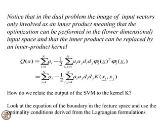
We therefore only need a suitable choice of kernel function cf:
Mercer’s Theorem:

Let K(x,y) be a continuous symmetric kernel that defined in the
closed interval [a,b]. The kernel K can be expanded in the form

Κ (x,y) = φ(x) T φ(y)

provided it is positive definite. Some of the usual choices for K are:

Polynomial SVM (x T xi+1)p p specified by user

RBF SVM exp(-1/(2σ2) || x – xi||2) σ specified by user

MLP SVM tanh(s0 x T xi + s1)

R
1 R R
k =1 2 k =1 l =1
R
Subject to these
constraints:
0 ≤ αk ≤ C ∀k ∑α
k=1
k yk = 0

Then define: Datapoints with αk > 0
R will be the support
w = ∑ k yk x k
α vectors classify with:
Then

k=1 f(x,w,b) = sign(w. x - b)
..so this sum only needs
b = y K (1 −ε K ) −x K .w K to be over the
support vectors.
k



1 

Constant Term Quadratic
 2 x1 


2 x2 
 Linear Terms
Basis
 : 

 2 xm  
Functions
 x12

 2  Pure Number of terms (assuming m input
 x2 
Quadratic dimensions) = (m+2)-choose-2
 : 
  Terms
xm2 = (m+2)(m+1)/2
 
Φ(x) = 
2 x1 x2  = (as near as makes no difference) m2/2
 
 2 x1 x3 
 : 
 
 2 x1 xm  You may be wondering what those
  Quadratic
 2 x2 x3 
Cross-Terms
2 ’s are doing.
 : 
  •You should be happy that they do no
 2 x1 xm  harm
 : 

 2x x  
•You’ll find out why they’re there
 m −1 m  soon.

QP with basis functions
R
1 R R
Maximize ∑ αk − 2 ∑∑ αk αl Qkl where Qkl = yk yl (Φ(x k ).Φ(xl ))
k =1 k =1 l =1

R
Subject to these
constraints:
0 ≤ αk ≤ C ∀k ∑α
k=1
k yk = 0

Then define:

w= ∑ k y k Φ( x k )
k s.t. α k >0 f(x,w,b) = sign(w. φ (x) - b)
b = y K (1 −ε K ) −x K .w K
k

QP with basis functions
R
1 R R
k =1 k =1 l =1
We must do R2/2 dot products to
get this matrix ready.
R
Subject to these 0 ≤ αk ≤ C ∀k product ∑ k m k = 0
Each dot
α y
requires /2 2
constraints: k= 1
additions and multiplications
The whole thing costs R2 m2 /4.
Then define:
Yeeks!

w= ∑ k y k Φ( x k )
α Then classify with: or does it?
…
b = y K (1 −ε K ) −x K .w K
k

 1   1  1
   
 2a1   2b1 
 +
2 a2   2b2 
    m

 :   :  ∑ 2a b i i
 2 am   2bm 
i =1
   
 a12
  b1 2
 +
 2   2 
 a2   b2  m

 :   :  ∑ ai2bi2
 2
  2
 i =1

 am   bm 
Φ(a) • Φ(b) = 

2a1a2 
•
 
2b1b2 

Quadratic
 2a1a3   2b1b3  +


:  
 
: 

Dot Products
 2a1am   2b1bm 
    m m

 2a2 a3   2b2b3  ∑ ∑ 2a a b b i j i j
 :   :  i =1 j =i +1
   
 2a1am   2b1bm 
 :   : 

 2a a   2b b 
  
 m −1 m   m −1 m 

Just out of casual, innocent, interest,
let’s look at another function of a and
Quadratic b:
(a.b + 1) 2
Dot Products = (a.b) 2 + 2a.b + 1
2
 m
 m
=  ∑ ai bi  + 2∑ ai bi + 1
 i =1  i =1

Φ(a) • Φ(b) = m m m
m m m m = ∑∑ ai bi a j b j + 2∑ ai bi + 1
1 + 2∑ ai bi + ∑ a b + ∑
2 2
i i ∑ 2a a b bi j i j
i =1 j =1 i =1
i =1 i =1 i =1 j =i +1
m m m m
= ∑ (ai bi ) + 2∑
2
∑a b a b i i j j + 2∑ ai bi + 1
i =1 i =1 j =i +1 i =1

Just out of casual, innocent, interest,
let’s look at another function of a and
Quadratic b:
(a.b + 1) 2
Dot Products = (a.b) 2 + 2a.b + 1
2
 m
 m
=  ∑ ai bi  + 2∑ ai bi + 1
 i =1  i =1

Φ(a) • Φ(b) = m m m
m m m m = ∑∑ ai bi a j b j + 2∑ ai bi + 1
1 + 2∑ ai bi + ∑ a b + ∑
2 2
i i ∑ 2a a b bi j i j
i =1 j =1 i =1
i =1 i =1 i =1 j =i +1
m m m m
= ∑ (ai bi ) + 2∑
2
∑a b a b i i j j + 2∑ ai bi + 1
i =1 i =1 j =i +1 i =1

They’re the same!
And this is only O(m) to
compute!

QP with Quadratic basis functions
R
1 R R
k =1 k =1 l =1
We must do R2/2 dot products to
get this matrix ready.
R
Subject to these 0 ≤ αk ≤ C ∀k product ∑ k y k = 0
Each dot
α
now only requires
constraints: k=1
m additions and multiplications

Then define:

w= ∑ k y k Φ( x k )
b = y K (1 −ε K ) −x K .w K
k

Higher Order Polynomials
Polynomial φ (x) Cost to build Cost if 100 φ (a).φ (b) Cost to Cost if
Qkl matrix inputs build Qkl 100
traditionally matrix inputs
efficiently
Quadratic All m2/2 m2 R2 /4 2,500 R2 (a.b+1)2 m R2 / 2 50 R2
terms up to
degree 2

Cubic All m3/6 m3 R2 /12 83,000 R2 (a.b+1)3 m R2 / 2 50 R2
terms up to
degree 3

Quartic All m4/24 m4 R2 /48 1,960,000 (a.b+1)4 m R2 / 2 50 R2
terms up to R2
degree 4

QP with Quintic basis functions
R R R
Maximize ∑ α + ∑∑ α α Q
k =1
k
k =1 l =1
k l kl
where Qkl = yk yl (Φ(x k ).Φ(x l ))

R
Subject to these
constraints:
0 ≤ αk ≤ C ∀k ∑α
k=1
k yk = 0

Then define:

w= ∑α
k s.t. α k >0
k y k Φ( x k )

b = y K (1 −ε K ) −x K .w K
Then classify with:
k f(x,w,b) = sign(w. φ (x) - b)

We must do RR/2 dot products to get this
2
R R

∑ α + ∑∑ α α Q
matrix ready.
Maximize k k l kl
In 100-d, each 1 product now needs 103
k = dot k =1 l =1
operations instead of 75 million
R
But there are still worrying things lurking away.
Subject to these
What are they?
constraints:
0 ≤ α ≤ C ∀k
k ∑α ky =0
k
•The fear of overfittingk = this enormous
with
1
number of terms
Then define: •The evaluation phase (doing a set of
predictions on a test set) will be very

∑
expensive (why?)
w= α k y k Φ( x k )
k s.t. α k >0

b = y K (1 −ε K ) −x K .w K
Then classify with:

2
R R

∑ α + ∑∑ α α Q
matrix ready.
Maximize k k l kl
k = dot k =1 l =1
The use of Maximum Margin
operations instead of 75 million magically makes this not a
problem R
Subject to these
What are they?
constraints:
0 ≤ α ≤ C ∀k
k ∑α ky =0
k
with
1
number of terms

∑
expensive (why?)
k s.t. α k >0 Because each w. φ (x) (see below)
needs 75 million operations. What
b = y K (1 −ε K ) −x K .w K can be done?
Then classify with:

2
R R

∑ α + ∑∑ α α Q
matrix ready.
Maximize k k l kl
k = dot k =1 l =1
The use of Maximum Margin
operations instead of 75 million magically makes this not a
problem R
Subject to these
What are they?
constraints:
0 ≤ α ≤ C ∀k
k ∑α k y =0
k
with
1
number of terms

∑
expensive (why?)
k s.t. α k >0 Because each w. φ (x) (see below)
needs 75 million operations. What
b Φ x ( ∑ ) − x ⋅Φ
w ⋅=(y) =1 −ε k y k Φ(xk ) .w( x)
K
α
K
k s.t. α k >0 K K
can be done?
Then classify with:
where ∑ k yk ( max α
=K = argx k ⋅ x +1) 5
α
k s.t. α k >0 k
k
Only Sm operations (S=#support vectors)
f(x,w,b) = sign(w. φ (x) - b)

R
1 R R
Maximize ∑ αk − 2 ∑∑ αk αl Qkl where Qthink:don’tyoverfit(as kmuch asxl ))
k =1 k =1 l =1 you’d
kl =
Why SVMs y k l (Φ x ).Φ(

No matter what the basis function,
there are really R up to R
only
Subject to these
constraints:
0 ≤ αk ≤ C ∀k ∑α Ry =0
parameters: α1, α2 .. αk, and usually
k
most are set to zero by the Maximum
k=1
Margin.

Then define: Asking for small w.w is like “weight
decay” in Neural Nets and like Ridge
Regression parameters in Linear
w= ∑α
k s.t. α k >0
k y Φ( x )
k k regression and like the use of Priors
in Bayesian Regression---all designed
to smooth the function and reduce
w ⋅Φ( x) = ∑
b = y (1 −ε ) −x .wαk y k Φ( x k ) ⋅Φ( x) overfitting.
K k s.t. α k >0
K K K
Then classify with:
∑
=K = argx k ⋅ x +1) 5
where k s.t. α >0k yk ( max αk
α
f(x,w,b) = sign(w. φ (x) - b)
k
k
Only Sm operations (S=#support vectors)

SVM Kernel Functions

• K(a,b)=(a . b +1)d is an example of an SVM
Kernel Function
• Beyond polynomials there are other very
high dimensional basis functions that can be
made practical by finding the right Kernel
Function
– Radial-Basis-style Kernel Function:
 (a − b)
2

K (a, b) = exp −
 
 σ, κ and δ are magic
 2σ 2  parameters that must
– Neural-net-style Kernel Function: be chosen by a model
K (a, b) = tanh(κ a.b − δ ) selection method
such as CV or VCSRM

SVM Implementations

• Sequential Minimal Optimization, SMO,
efficient implementation of SVMs, Platt
– in Weka
• SVMlight
– http://svmlight.joachims.org/

References

• Tutorial on VC-dimension and Support
Vector Machines:
C. Burges. A tutorial on support vector machines for
pattern recognition. Data Mining and Knowledge
Discovery, 2(2):955-974, 1998.
http://citeseer.nj.nec.com/burges98tutorial.html
• The VC/SRM/SVM Bible:
Statistical Learning Theory by Vladimir Vapnik, Wiley-
Interscience; 1998

Svm

More Related Content

What's hot

Similar to Svm

Recently uploaded

Svm

Editor's Notes