CBM Variable Speed Machinery

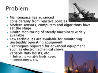
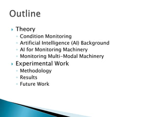
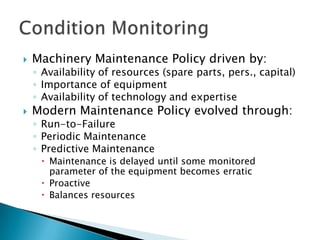
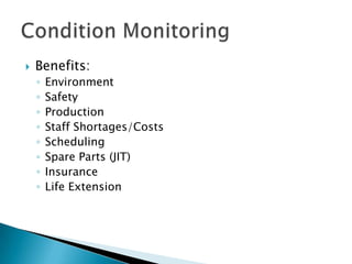
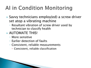
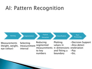
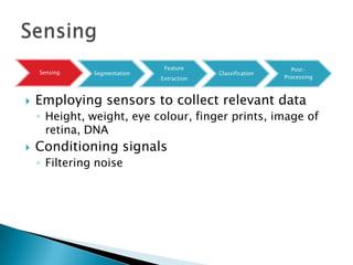
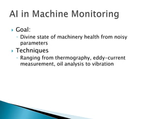
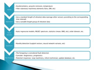
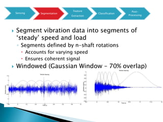
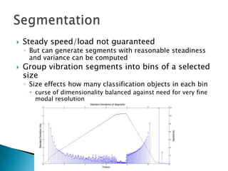
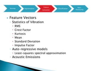
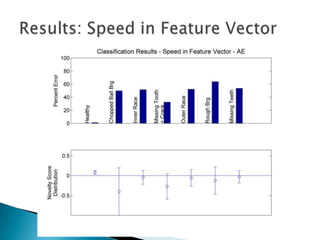
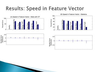
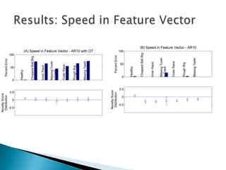
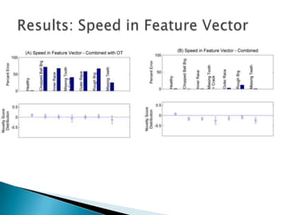
As submitted to Mechanical Systems and
Signal Processing

Jordan McBain, P.Eng.

 Maintenance has advanced
considerably from reactive policies
 Modern sensors, computers and algorithms have
set the stage
 Health Monitoring of steady machinery widely
available
 Few techniques are available for monitoring
unsteadily operating equipment
 Techniques required for advanced equipment
such as electromechanical shovel,
variable duty hoists, etc.
◦ Subject to variable loads, speed,
◦ temperatures, etc.

 Theory
◦ Condition Monitoring
◦ Artificial Intelligence (AI) Background
◦ AI for Monitoring Machinery
◦ Monitoring Multi-Modal Machinery
 Experimental Work
◦ Methodology
◦ Results
◦ Future Work

 Machinery Maintenance Policy driven by:
◦ Availability of resources (spare parts, pers., capital)
◦ Importance of equipment
◦ Availability of technology and expertise
 Modern Maintenance Policy evolved through:
◦ Run-to-Failure
◦ Periodic Maintenance
◦ Predictive Maintenance
 Maintenance is delayed until some monitored
parameter of the equipment becomes erratic
 Proactive
 Balances resources

 Benefits:
◦ Environment
◦ Safety
◦ Production
◦ Staff Shortages/Costs
◦ Scheduling
◦ Spare Parts (JIT)
◦ Insurance
◦ Life Extension

 Savvy technicians employ(ed) a screw driver
set atop a vibrating machine
◦ Resultant vibration of screw driver used by
technician to classify health
 AUTOMATE THIS!
◦ More sensitive
◦ Earlier detection of faults
◦ Consistent, reliable measurements
 Consistent, reliable classification

 One branch of artificial-intelligence domain
 Usually involves representing a state or object
to be indentified with a vector of
commensurate numerical values
 Representative vector called a “pattern” or
“classification object”
 Classification achieved by computing decision
surfaces around classes of objects

 Example: biometric classification of
employees reporting to work

Feature Post-
Sensing Segmentation Classification
Extraction Processing

Measurements Selecting Reducing Plotting -Decision Support
(height, weight, measurement segmented values in -Also detect
eye colour) interval measurements n-dimensions enebriation
to key and fitting a -Pay
numbers boundary -Etc.

Feature Post-

 Employing sensors to collect relevant data
◦ Height, weight, eye colour, finger prints, image of
retina, DNA
 Conditioning signals
◦ Filtering noise

Feature Post-

 Sensor data divided into useful chunks
◦ Separate employees from one another
 Use a terminal for employees to sign in one at a time
 Use image processing and separate employees from
each other in picture
 One of the most difficult problems in pattern
recognition

Feature Post-

 Characterizes an object to be recognized by
measurements whose values are very similar for
objects in the same category
 Invariant to irrelevant transformations
 An ideal feature vector makes the job of
classification trivial (e.g. DNA)
 The curse of dimensionality
◦ A balance between improvements from increased
dimensionality and increased need for data to describe
the space and added complexities

Feature Post-

 Employs full feature vector provided by the
feature extractor to assign the feature vector‟s
object to a category
 Generalization – learning from a training set
extends well to unexperienced data
 E.g. Neural Networks
◦ As one would fit a model to an experimental data set
with least-squares regression, in classification one
would fit a boundary around a class‟ data set
◦ Computationally equivalent tasks
 But in classification, the problem is non-linear

Feature Post-

 Perform some action subsequent to
classification
 Improve classification error based on context
◦ Employ multiple classifiers

 Goal:
◦ Divine state of machinery health from noisy
parameters
 Techniques
◦ Ranging from thermography, eddy-current
measurement, oil analysis to vibration

• Accelerometers, acoustic emission, temperature
• Filter stationary machinery elements (fans, EMI, etc)
Sensing

• Use a standard length of vibration data (average other sensors according to the corresponding
time interval)
Segmentation • Use a variable length group of vibration data

• Auto-regressive models, MUSIC spectrum, statistics (mean, RMS, etc), order domain, etc.
Feature
Extraction

• Novelty detection (support vectors, neural network variants, etc)
Classification

• The foregoing is considered fault detection
• Consider: diagnostics, prognostics
Post-Processing • Potential responses: stop machinery, inform technician, update database, etc.

 Heavily used in literature
 Non-destructive, online, sensitive
 Faults in rotating machinery have
strongly representative features
in the frequency domain
 Consider bearings:
◦ Frequency Response a function of
Fault, Slippage, Noise

Diagrams from: Randall, B. State
of the Art in Machinery Monitoring, JSV

 Motivation: addresses imbalance of data from
one class in relation to that of others
◦ Data from faulted states are difficult to collect
(economics, operation)
 Sub problem of pattern recognition
◦ train on the “normal” class and then signal error when
behaviour deviates from itDecision boundary encircles
normal patterns
 A wide variety of techniques available
 Examine two:
◦ Boundaries containing a certain quantile of data (i.e. a
discordance test)
◦ Boundaries derived by Support Vectors

 Support Vector Technique: Tax‟s Support
Vector Data Description (for Novelty
Detection)
◦ Attempts to fit a sphere of minimal radius around
normal data
◦ But a in a higher dimensional space (using the
“kernel trick”)
 Generates a very flexible decision boundary in the
input space

 Simplest machine
◦ damped spring system

 
mx cx kx f (t ) k c
n
m 2 km
◦ Frequency domain representation
1 1
H ( w) 2
m wn w2 j 2 wn w

◦ Forced with a function f (t ) A *sin( 0t )

 With frequency-domain representation
A A
F( ) ( 0) ( 0 )
2 2

 The system‟s output is given by X ( ) F ( )H ( )
1 1 A A
X( ) 2 2
( ( 0) ( 0 ))
m wn w0 j 2 wn w0 2 2

 Underground mines
◦ Ventilation fans driven with VFD to optimize
efficiency
◦ Fans driven at one speed one day and then changed
to a different constant speed
 New forcing function

A2 sin( 1t ), t 0
f (t )
A3 sin( 2t ), t 0

 Examine function for one day (windowing)
t
f (t ) rect ( )* A4 sin( 3t )
 Frequency representation (convolution
operator):

A A
F( ) Rect( ) ( ( 3) ( 3 ))
2 2
A A
sinc( ) ( ( 3 ) ( 3 ))
2 2
A
(sinc( 3 ) sinc( 3 ))
2

 System‟s response to forcing, similar
◦ Spectral leakage and smearing by windowing

 Consider function including instant of change
for a period of time 2*Tow
t 1 t 1
f (t ) rect (2 )* A2 sin( 1t ) rect (2 )* A3 sin( 3t )
2 2
 Resultant frequency representation
A1 A1 A2 A2
F( ) Rect( ) ( ( 1) ( 1 )) Rect( ) ( ( 2) ( 2 ))
2 2 2 2 2 2 2 2
A A
(sinc( 1) sinc( 1 )) (sinc( 2 ) sinc( 2 ))
4 4

 Sinc functions with sidelobes
◦ Introducing interference on spectrum
◦ Central frequencies contaminated with frequency
info from windowing function
◦ Info not solely indicative of health

 Forced function with time varying frequency
f (t ) Ac cos(2 f ct cos(2 f mt ))
◦ f m as modulating frequency
◦ f c as carrier frequency
◦ modulation index
 No closed form solution of fourier integral
 Use bessel functions

 (Mathematically) unlimited bandwidth
 In practice 98% of bandwidth determined by
beta

 Examining over a period of time (windowing)
◦ Introduces sinc functions mounted on impulses
◦ Consequence: spectral interference
 Conclusion
◦ Frequency domain contains valuable info on:
 System behaviour
 Faults manifested in the form of changes in stiffness and
damping
 Forcing function
◦ Info in frequency bands not limited to system
behaviour

 Gear interaction modeled with:
 
mx cx kx f (t )
 As suggested by
J- Kuang, A- Lin. Theoretical aspects of Torque responses in spur
gearing due to mesh stiffness variation, Mechanical Systems and
Signal Processing. 17 (2003) 255-271.
 Assume
◦ Fixed load of L (Nm)
◦ Damping ratio of c=0.17
◦ Spring value k = k(t)
 Normal assumptions of spring constant
◦ Clean frequency plot
◦ Obvious harmonics and sidebands

 Spring stiffness varies with time

 Consequence: non-linear frequency response
◦ Convolution introduced
2
m X ( ) cj X ( ) K ( ) X( ) F( )

 Frequency response of k(t), modeled as simple
pulse train, is well known (RADAR, SONAR)
◦ Sync function as envelop to impulse train
 Variable speed machinery
◦ Stiffness: variable pulse train
◦ I.e. Pulse Width Modulation
◦ No closed form Fourier integral
 Bessel functions
◦ Transfer function not discernible
 Numerical analysis necessary
 Consequence
◦ Spectrum incredibly complex
◦ No simple band to monitor

 Primary aggravators: load and speed
◦ Referred to as nuisance variables in the literature
 In vibration monitoring
◦ Power of vibration a product of the effects of load and
speed
 Relation between power and speed non-linear
 Resonances!
 Vibration a function of health and speed
 Complex machinery an amalgamation of spring-like elements
 Vibration in most mechanical systems involves periodic
oscillation of energy from potential to kinetic (according to
frequency response of spring approximation)
 When machine is healthy, deviations in consequent vibrations
are small

 When machine is healthy, deviations in consequent
vibrations are small
 When health is poor, deviations due to speed become
significant
 Stack: Damping in undamaged machinery is largely
insensitive to speed/load changes – damaged
machinery is not

Feature Post-

 Segment vibration data into segments of
„steady‟ speed and load
◦ Segments defined by n-shaft rotations
 Accounts for varying speed
 Ensures coherent signal
 Windowed (Gaussian Window – 70% overlap)

 Steady speed/load not guaranteed
◦ But can generate segments with reasonable steadiness
and variance can be computed
 Group vibration segments into bins of a selected
size
◦ Size effects how many classification objects in each bin
 curse of dimensionality balanced against need for very fine
modal resolution

Feature Post-

 Feature Vectors
◦ Statistics of Vibration
 RMS
 Crest Factor
 Kurtosis
 Mean
 Standard Deviation
 Impulse Factor
◦ Auto-regressive models
 Least-squares spectral approximation
◦ Acoustic Emissions

 Signal processing technique
◦ Not a feature vector
◦ Not a fault detection technique
 Resamples data at constant angular shaft intervals
◦ Rather than constant time intervals
 Tachometers employed (2500 pulses per rev)
 At max speed (500 rpm)
◦ 18 000 samples collected
◦ Tach pulses: 37 500 samples
 up-sampling x2 required
 At lowest speed (20 rpm)
◦ 450 000 samples collected
◦ Tach pulses: 112 500
 Up-sampling x4 required
 Up-sampling in the context of noise?

Feature Post-

 Thrust: Feature vectors are grouped according to
speed and a statistical model fit as function of
speed
 Motivation: Effects of machinery resonances
managed by subdividing novelty detection
 Limitations: Double curse of dimensionality,
assumption of Gaussianaity
 Contribution:
◦ Application to real world (machinery) data
◦ Evaluated theoretical limitations with respect to
machinery
◦ Improved approach by suggesting whitening first
followed by normal novelty detection

 Variable speed machinery
◦ Elements of a machine‟s vibratory response are
assumed to have a strong relation to the speed of
the given machinery
 Distribution for speeds:
◦ Means vary with speed *C30

◦ Variances vary with resonance response

*C20
y

* C10

x

 Thrust: One mode is included in the feature vector
which are grouped into bins according to ranges of
other mode (then employ multi-novelty detector
dispatch)
 Motivation: Advance the technique to higher modes
 Limitations: Curse of dimensionality, large number of
modes impractical, brute force
 Contribution:
◦ Very practical technique compared to literature (for load
and speed)
◦ “Crossing” modes to enhance classification results
 Experimental Data: Laurentian‟s TVS
 Status: Not yet validated

 Approach so far only works with one mode
 Employ Timusk‟s novelty detector dispatch
technique
◦ Routine
 Segment data into load bins
 For each load bin build a uni-modal novelty detector
for all speed data in that load bin
◦ Improve results
 Also build multiple detectors but based on speed bins
 Combine classification results

 Averaging modes still a problem
◦ Employ previous improvements
 Curse of dimensionality increases
◦ Some mitigation possible
 Brute force
◦ Across of the spectrum of techniques, not as bad as
parzen windowing (enter dataset is memorized)
 Higher number of modes increases
computational complexities and curse of
dimensionality

 Must account for speed!
 Worden‟s Statistical Parameterization
◦ Good results
◦ Subject to double curse of dimensionality and
gaussianaity
 Multi-Modal Novelty Detection
◦ Results on par or better than Worden‟s
◦ Somewhat insensitive to double curse of dimensionality
 Feature vectors
◦ Statistics poor
 Consequently, AE poor
◦ AR models produced excellent results
◦ Order Tracking poor
 Why?

 Thesis
◦ Multi-Modal Novelty Detection for Higher No.
Modes
◦ System Identification
 No need to account for modes in novelty detection
 Curse of dimensionality?
◦ Cross-Correlation
 No need to measure modes
 Silver bullet?
◦ Software Architecture

 CEMI
 Dr. Mechefske (Queens)
 Dr. Timusk
 Greg Lakanen
 Greg Dalton

CBM Variable Speed Machinery

More Related Content

Similar to CBM Variable Speed Machinery

CBM Variable Speed Machinery