Download to read offline
![ HSIC is the norm of a cross-covariance matrix
in kernel space.
2
HSIC (x, y) c xy
HS
C xy E xy [( ( x) x ) ( ( y) y )]
Empirical estimate of HSIC
1 s.t.
HSIC( X , Y ) : 2 tr (KHLH )
n H, K, L R n n ,
K ij : k ( xi , x j ), L ij : l ( yi , y j )
Number of
observations 1 T
H I 1n1n
n
Kernel functions](https://image.slidesharecdn.com/icmlpresentationv5-120926183554-phpapp02/75/2010-ICML-10-2048.jpg)
![ Cluster the features using spectral clustering.
Data x = [f1 f2 f3 f4 f5 …fd]
Feature similarity based on HSIC(fi,fj).
Transformation Matrix
f1 f2
… Wv
f4 1 0 0 . .
0 1 0 . .
f15 f34 f21 0 0 0 . .
… f3 …
f7 f9
0 0 1 . .
. . 0 . .](https://image.slidesharecdn.com/icmlpresentationv5-120926183554-phpapp02/75/2010-ICML-13-2048.jpg)
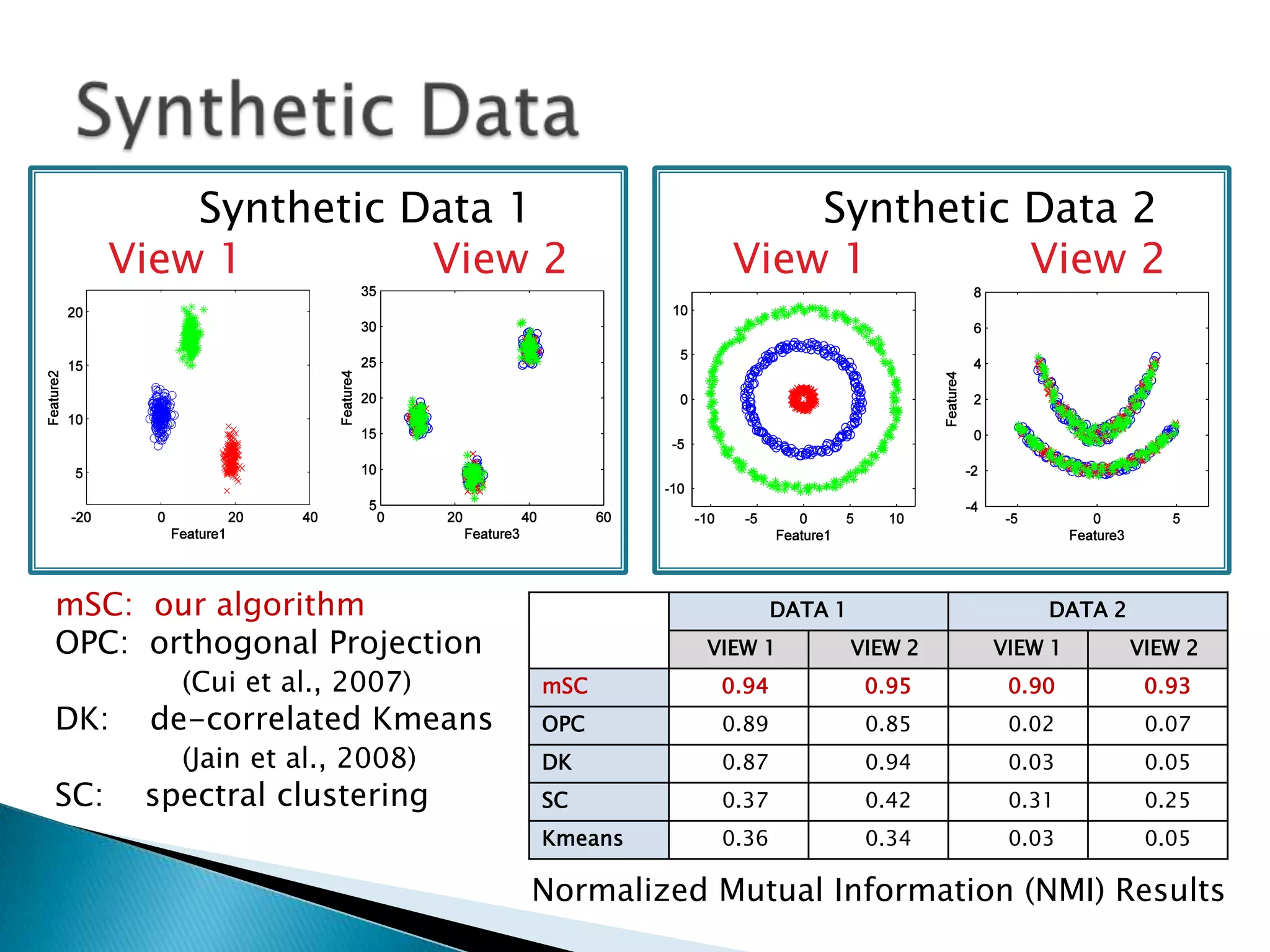
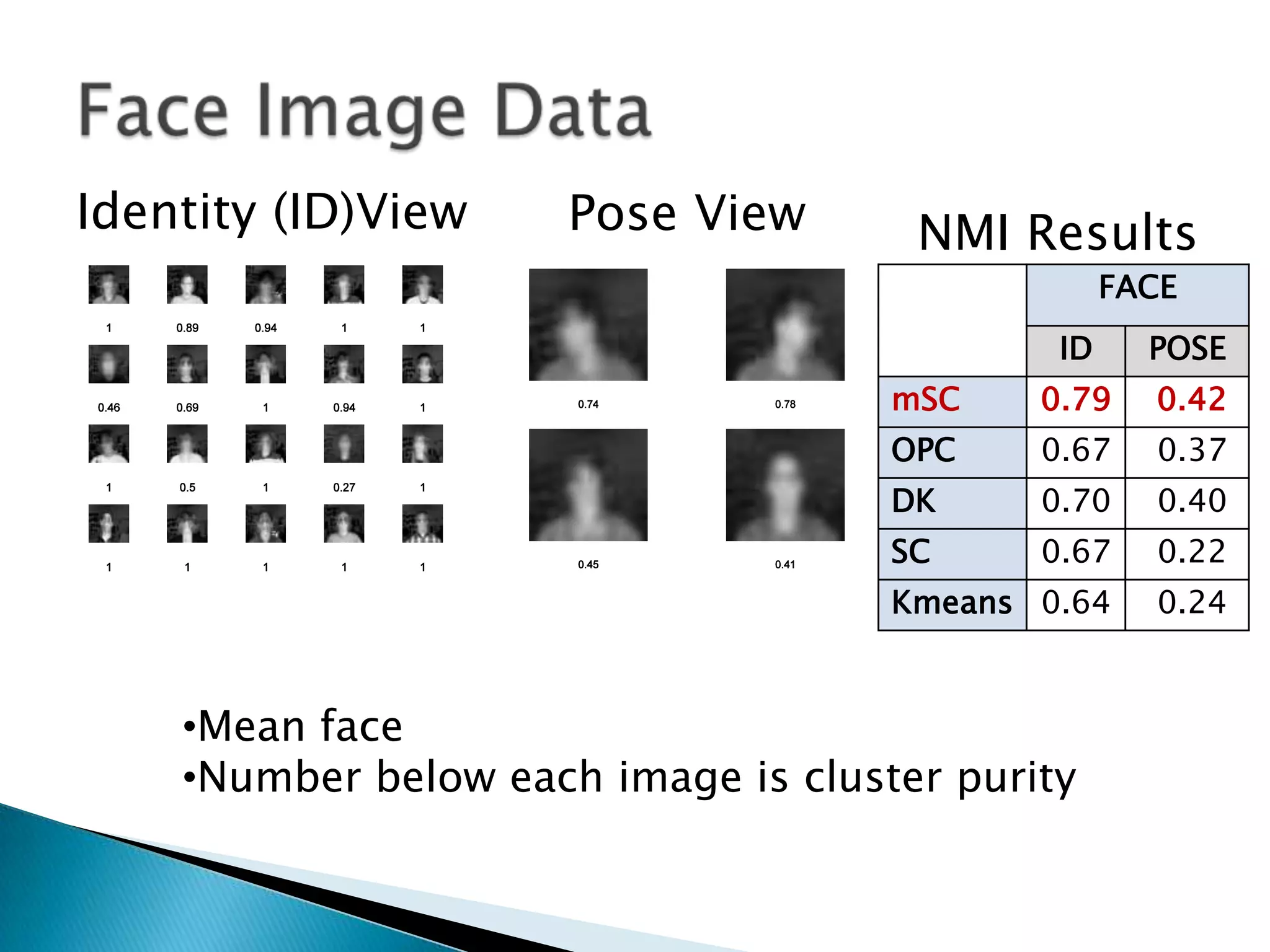
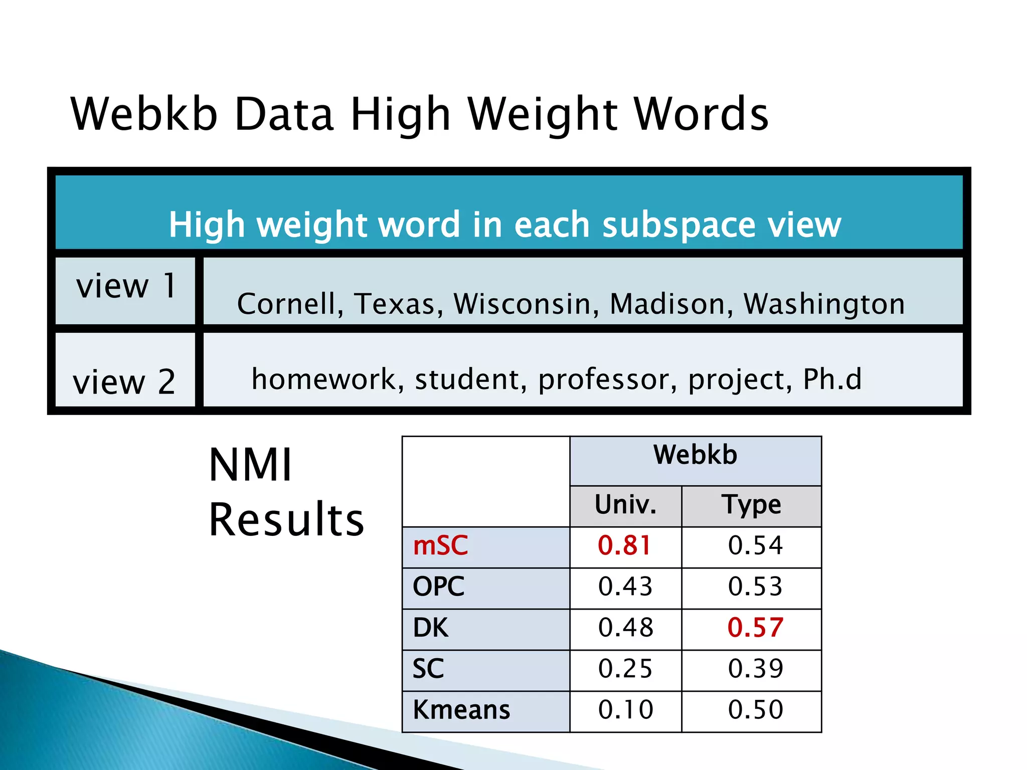
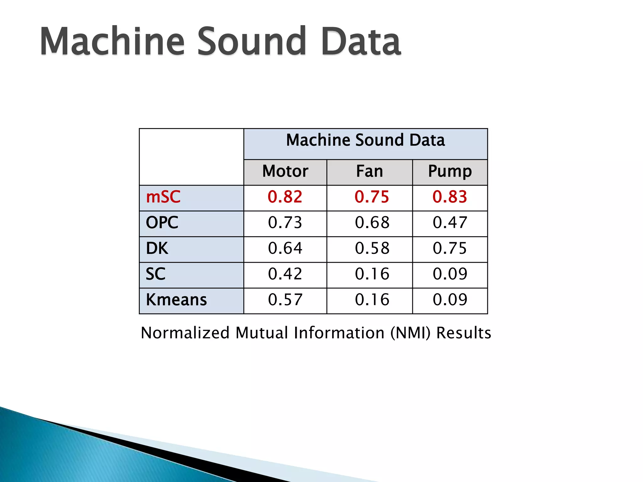


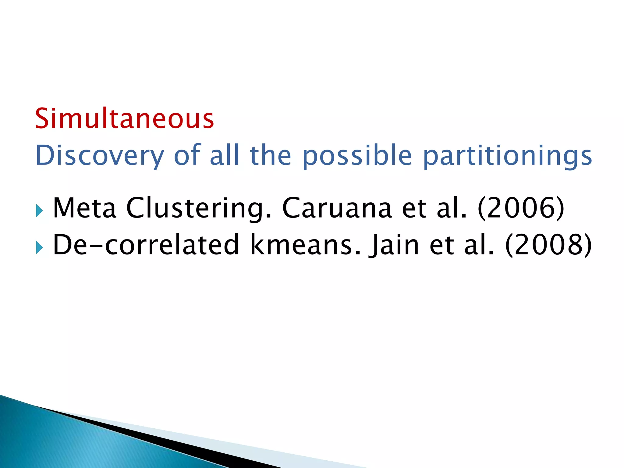
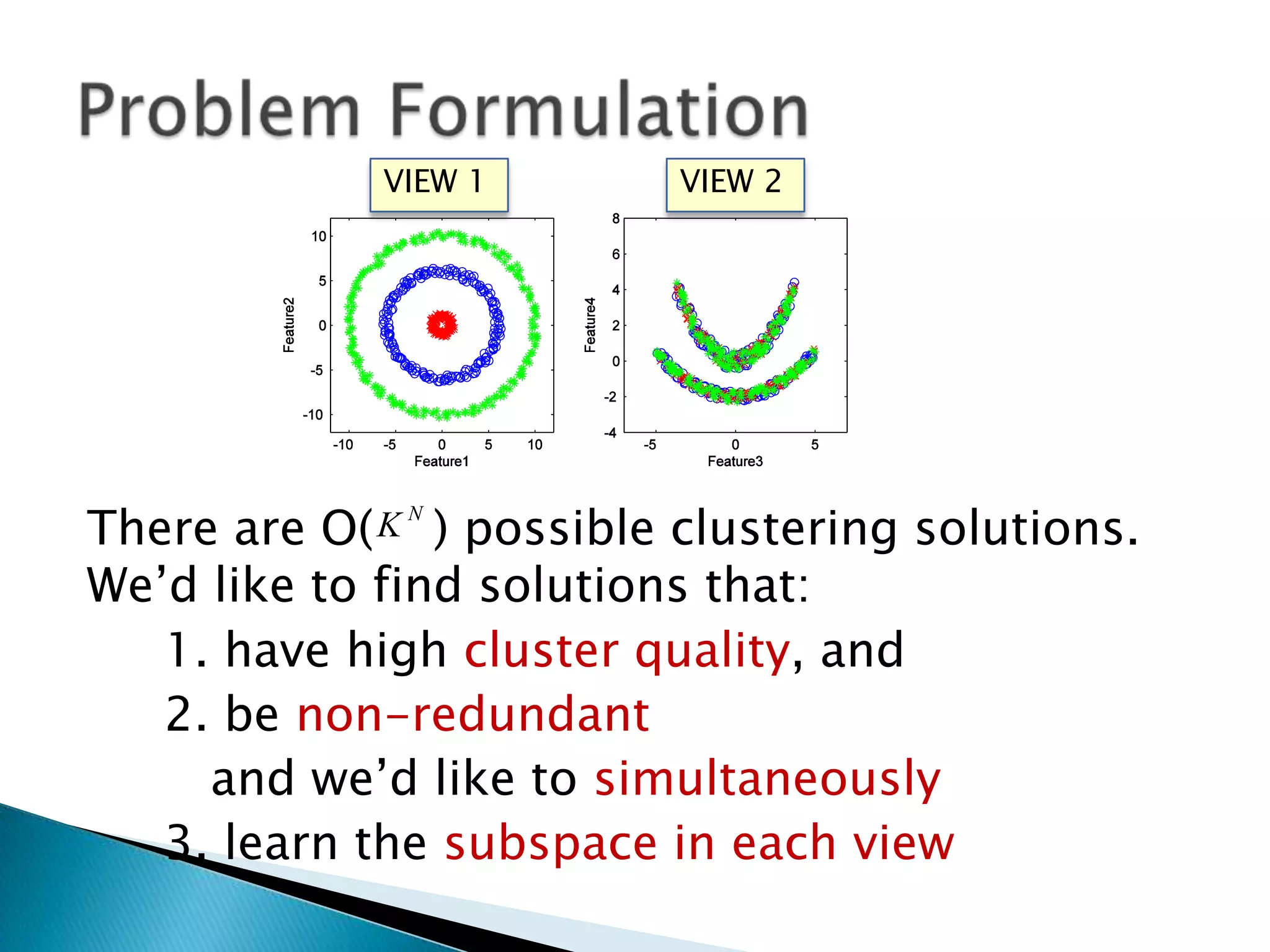
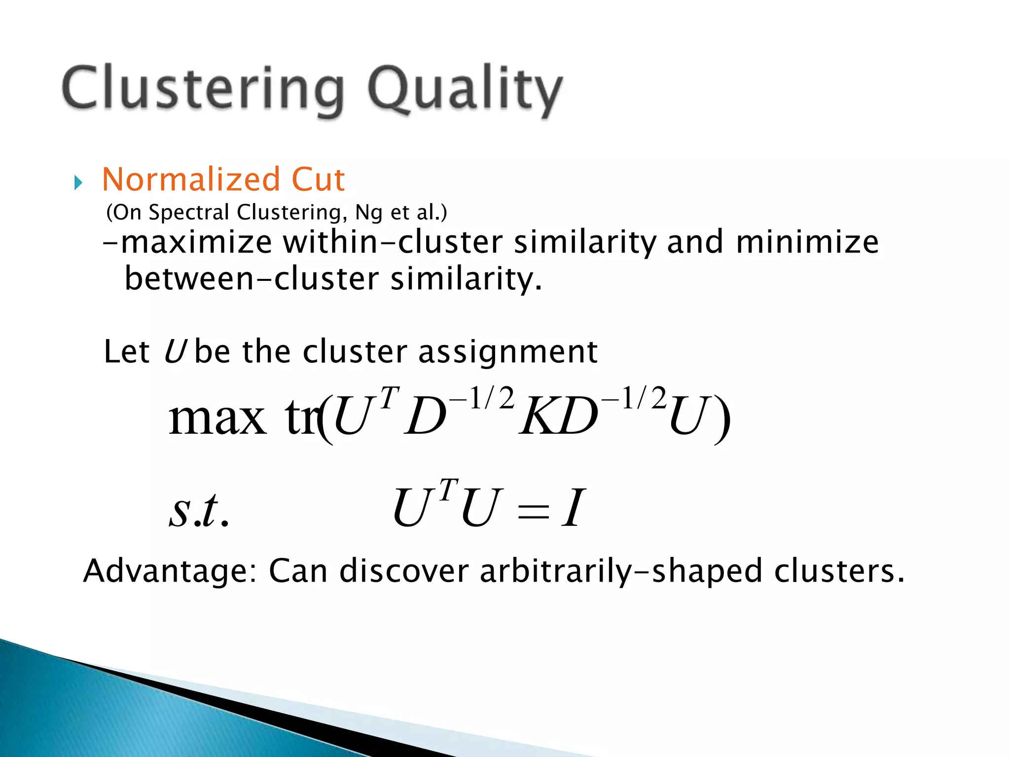
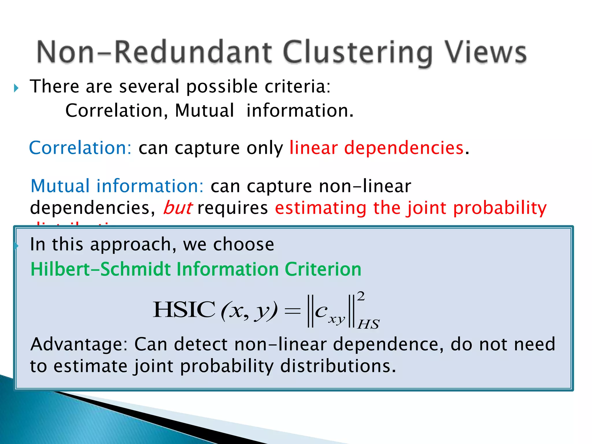
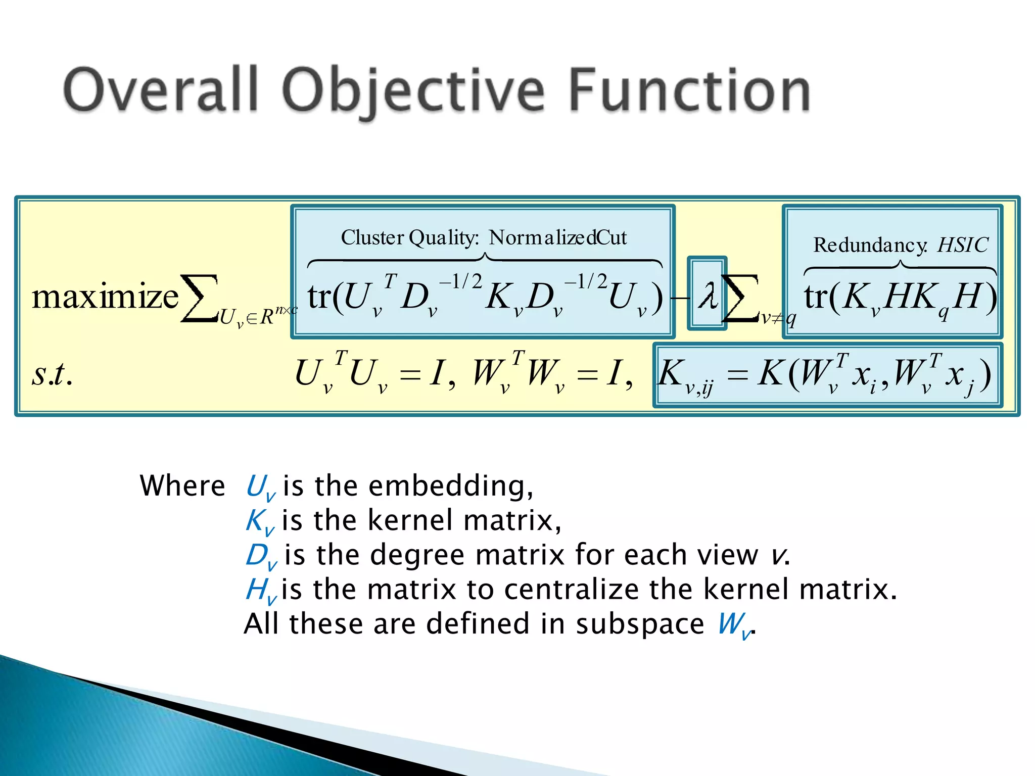
This document presents a new method called multi-view spectral clustering (mSC) for discovering multiple non-redundant clusterings from multi-view data. mSC optimizes both a spectral clustering objective to measure cluster quality and a Hilbert-Schmidt independence criterion regularization to measure redundancy between clusterings. It can discover clusters with flexible shapes while simultaneously learning the subspace for each clustering view. The method is evaluated on several datasets and is shown to outperform other multi-view clustering algorithms in terms of normalized mutual information.


![Vibe Coding vs. Spec-Driven Development [Free Meetup]](https://cdn.slidesharecdn.com/ss_thumbnails/vibecodingvsspecdrivendevelopment-251209105622-43f455e7-thumbnail.jpg?width=640&height=640&fit=bounds)


![Coded Agents – with UiPath SDK + LangGraph [Virtual Hands-on Workshop]](https://cdn.slidesharecdn.com/ss_thumbnails/codedagentsdeck-251215155422-5497c599-thumbnail.jpg?width=640&height=640&fit=bounds)


