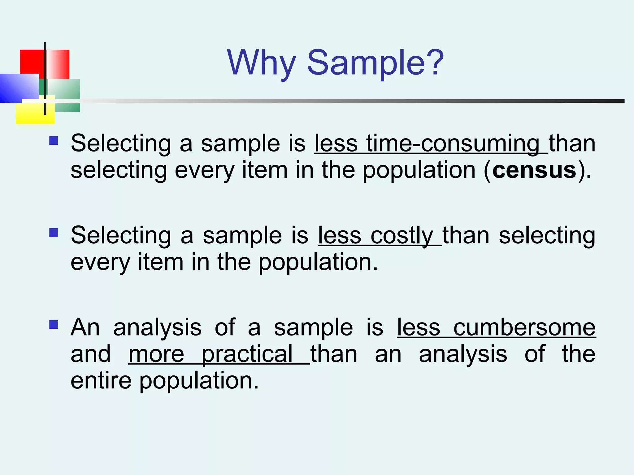
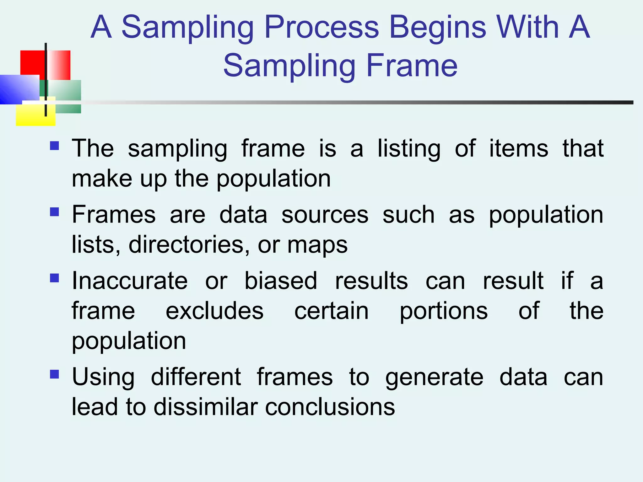
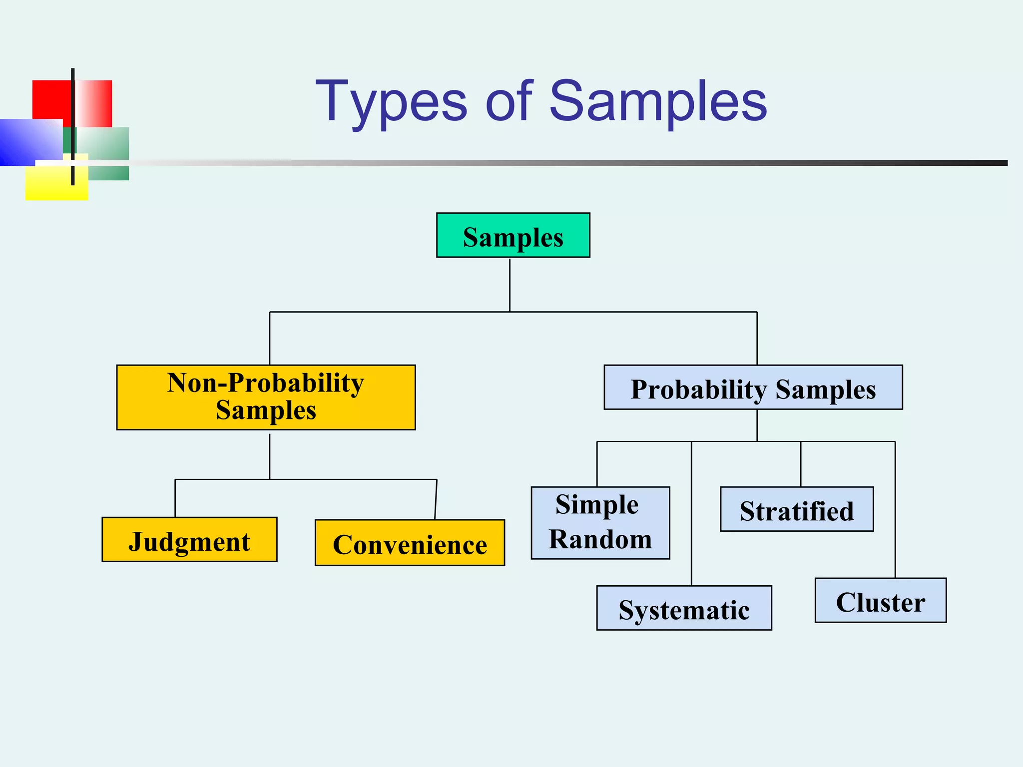
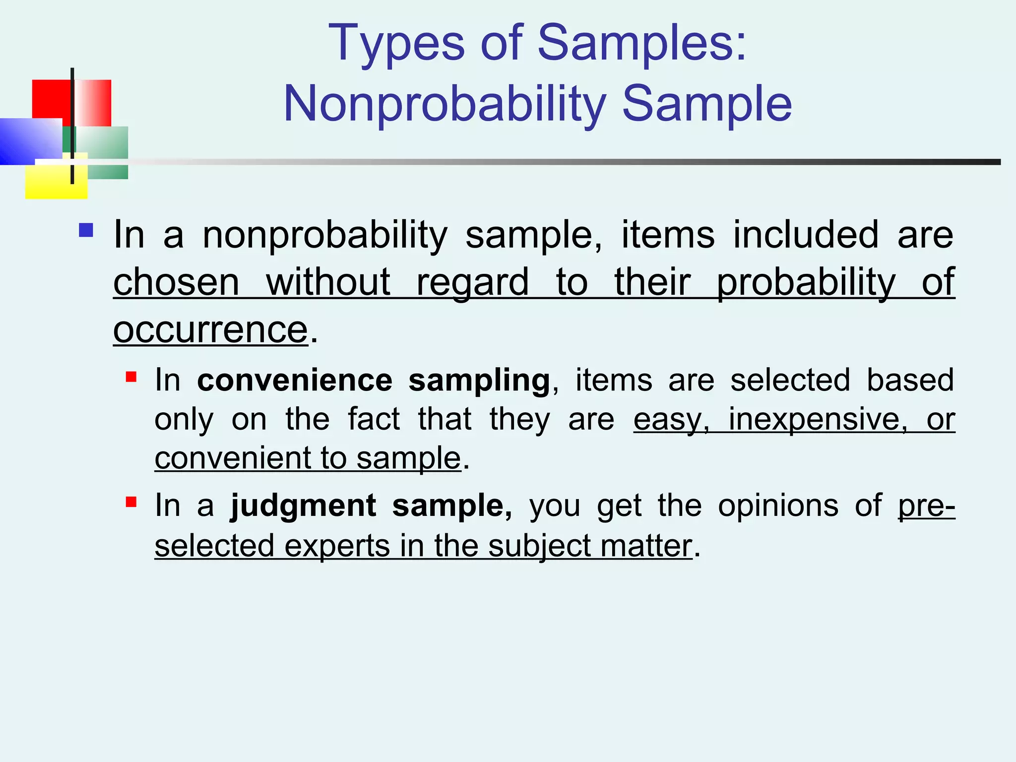
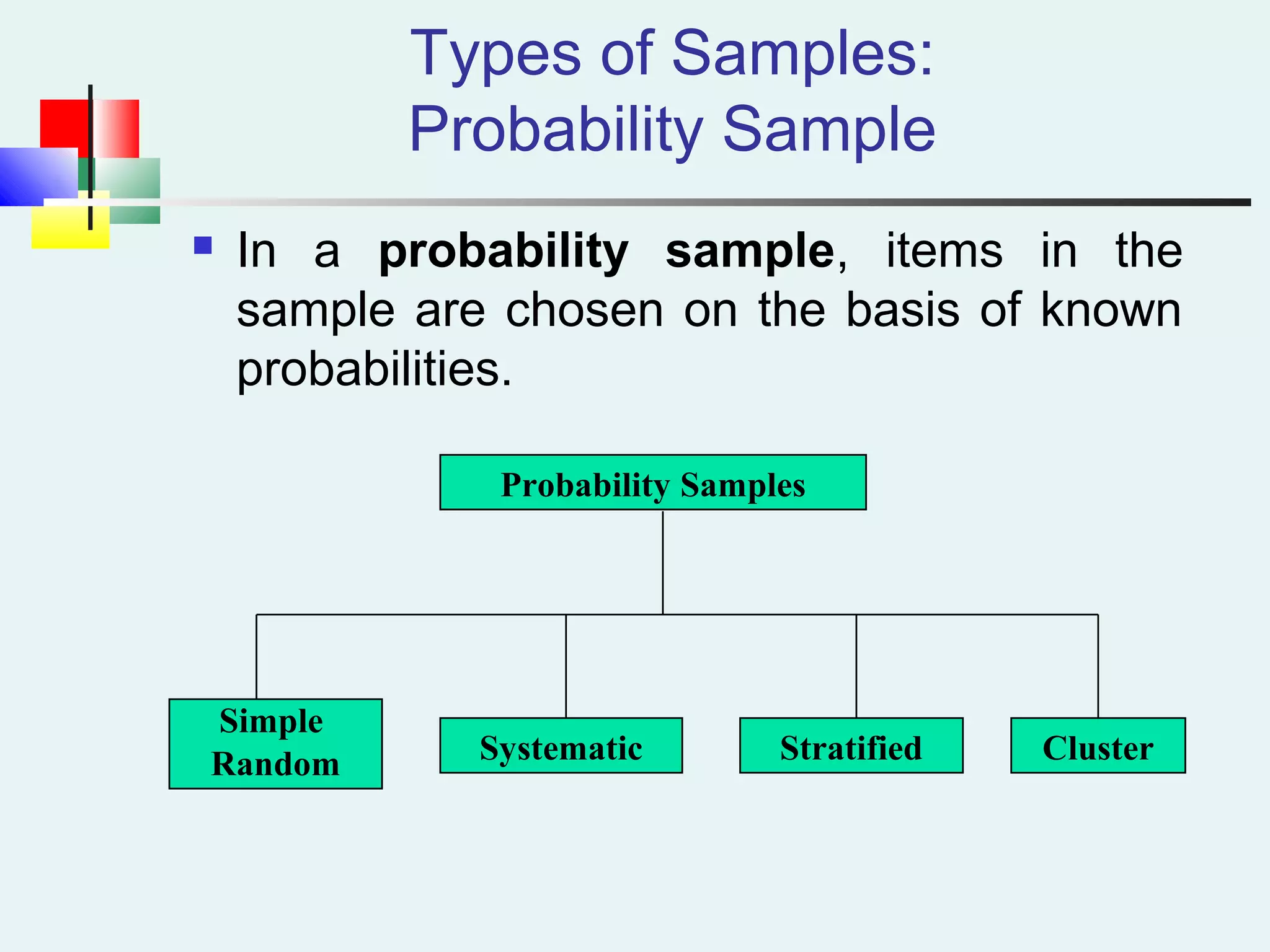
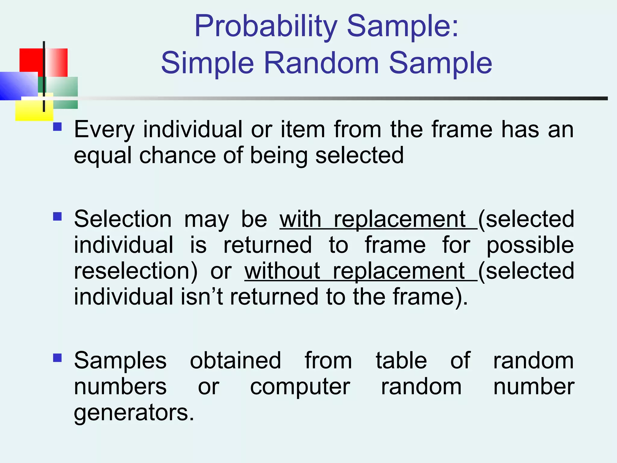
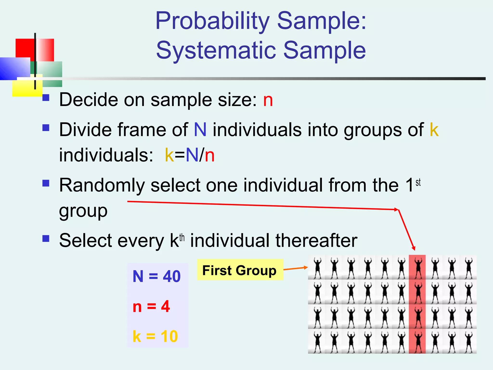
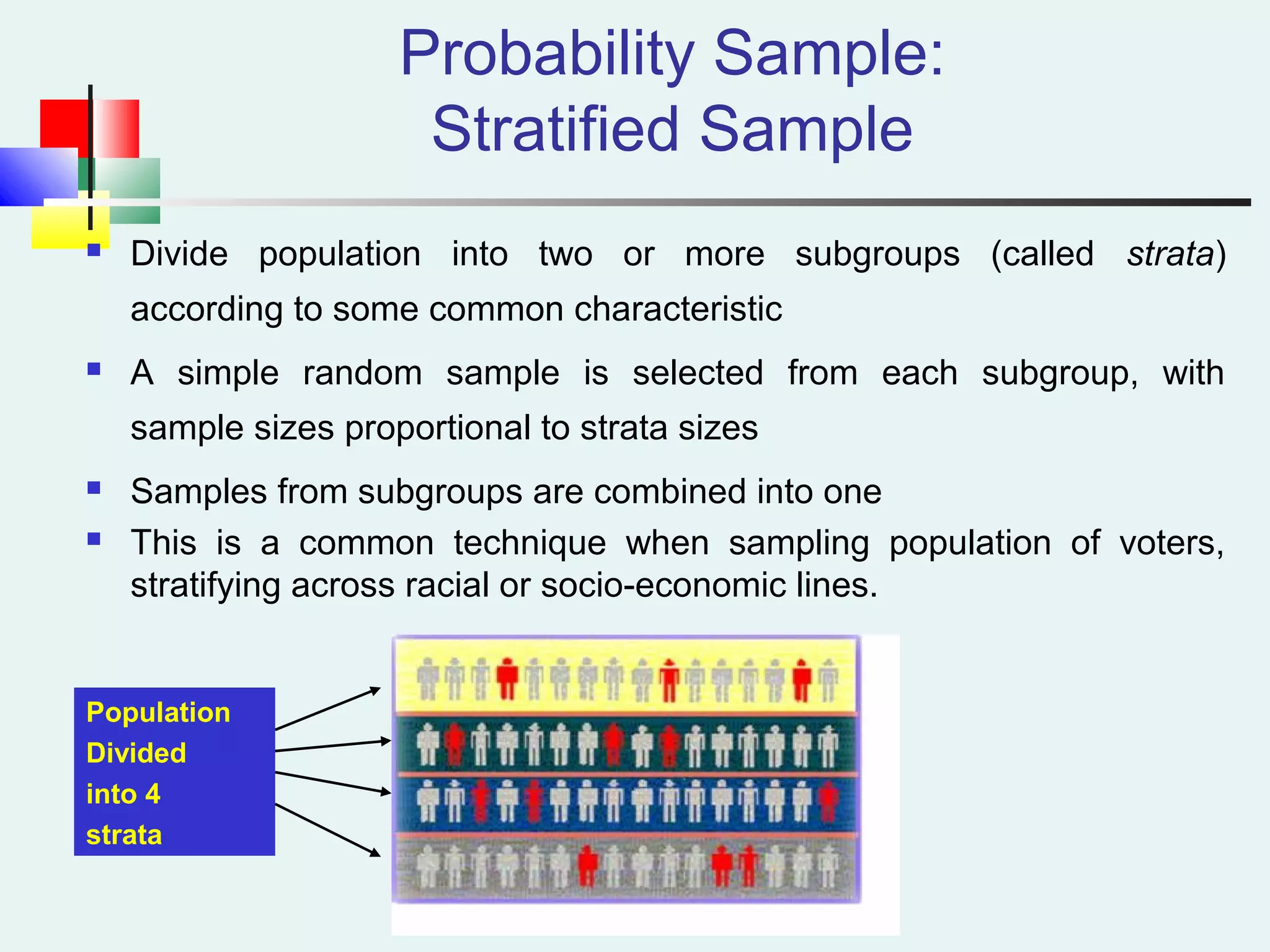
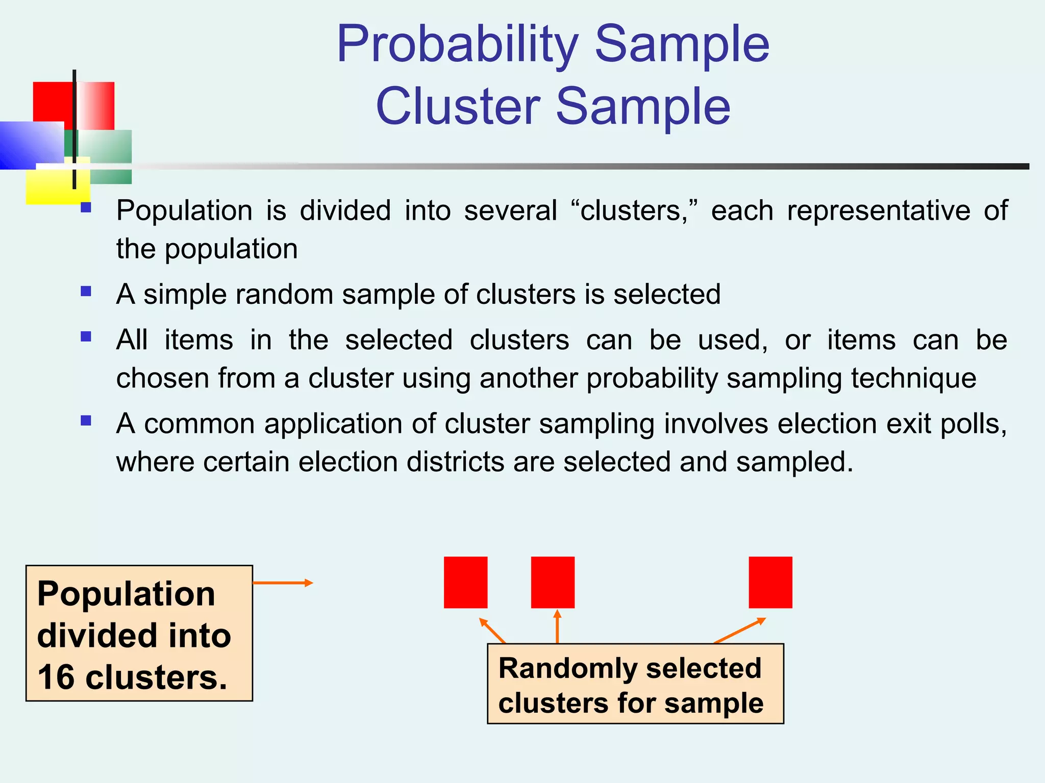
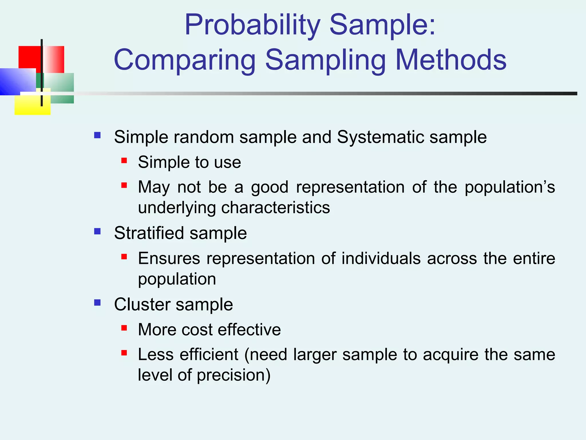
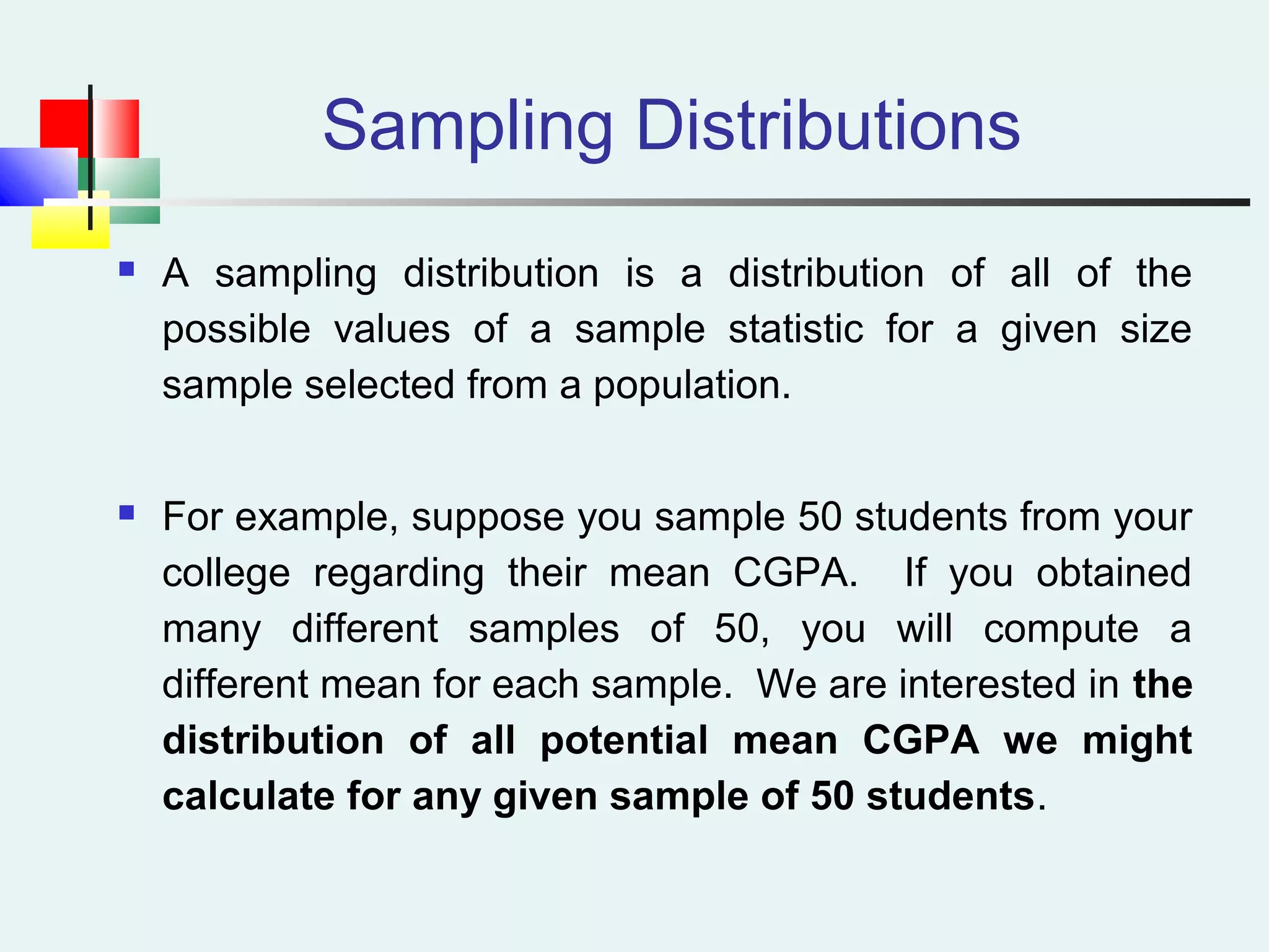
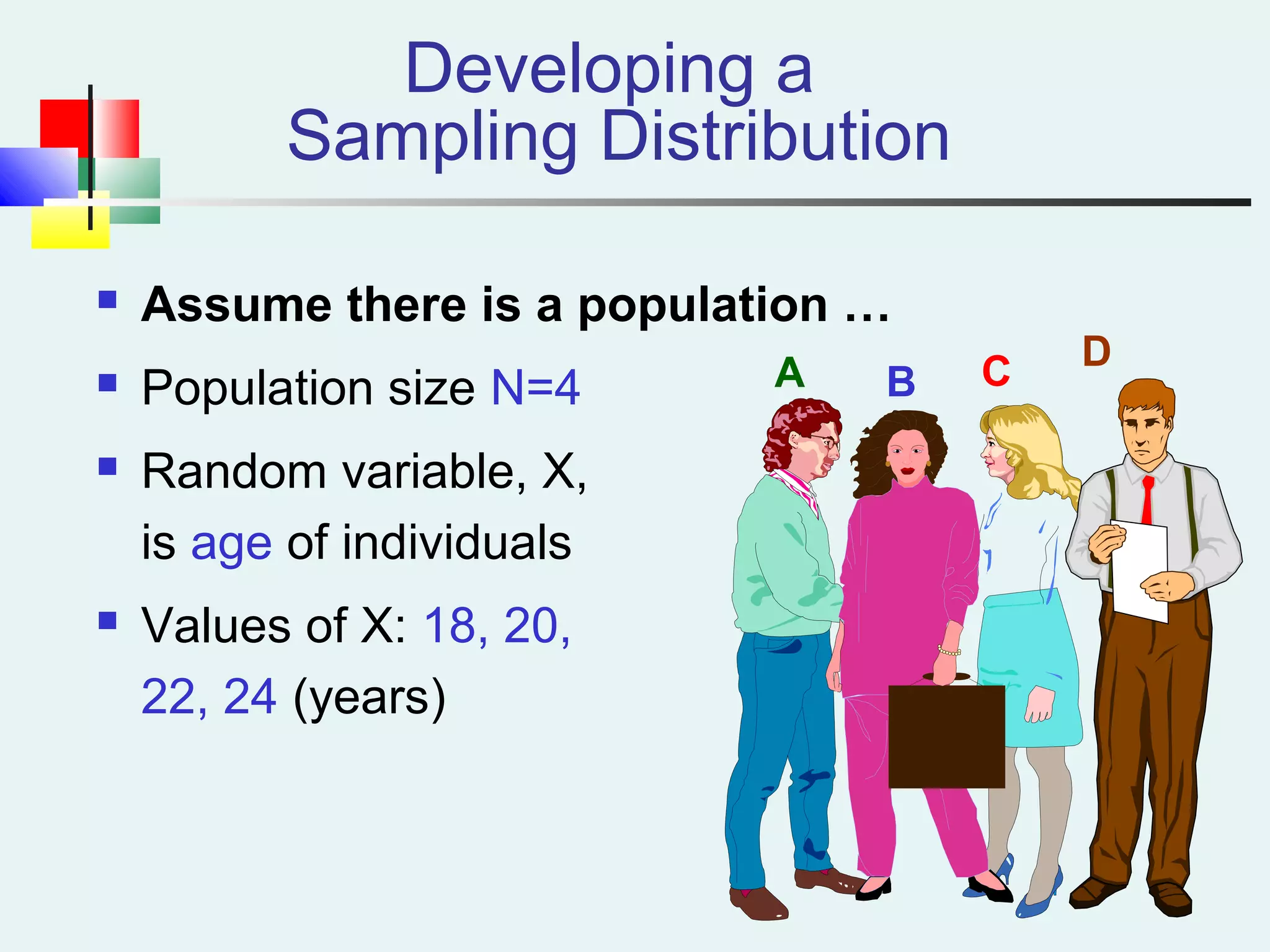
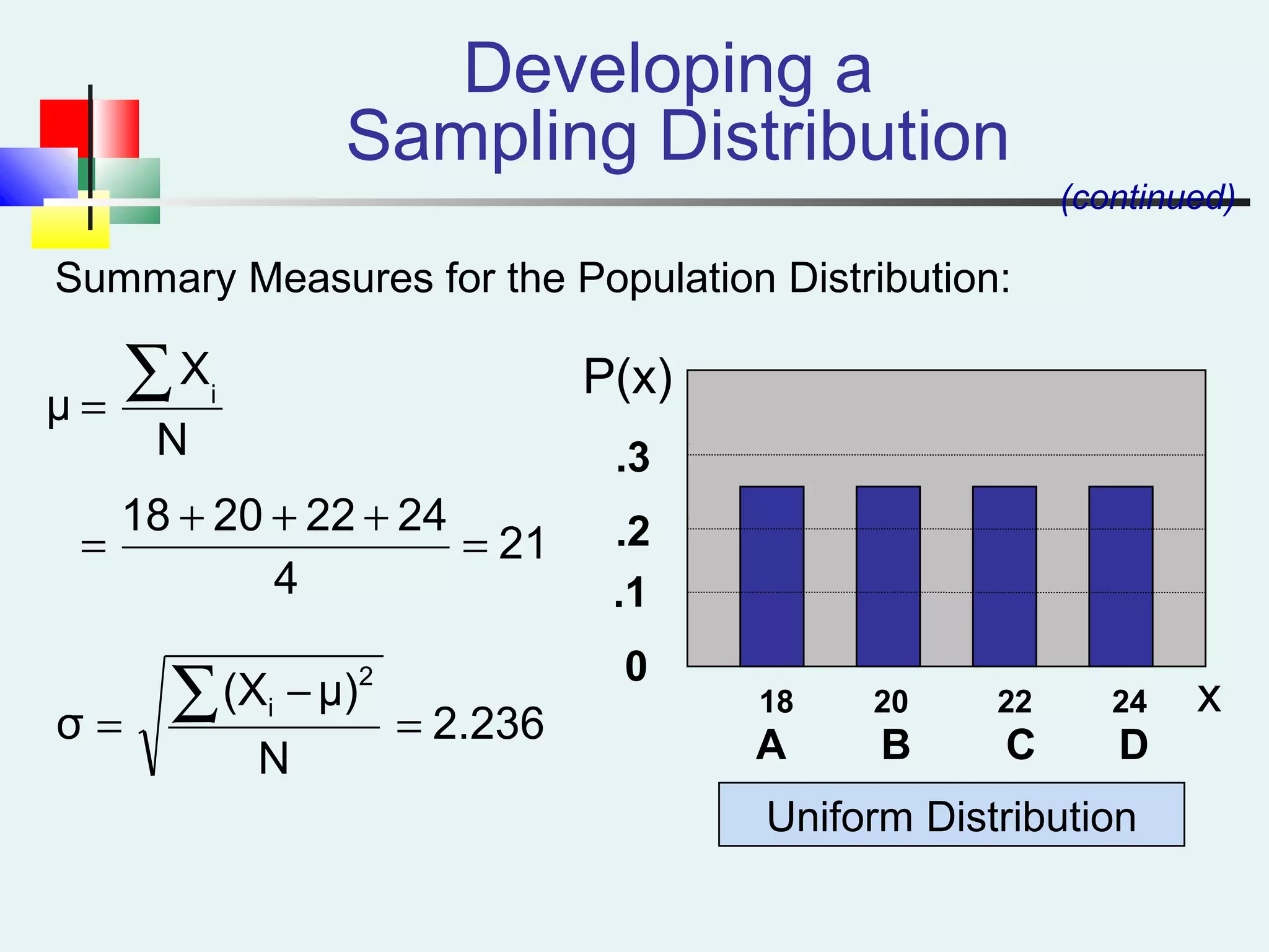
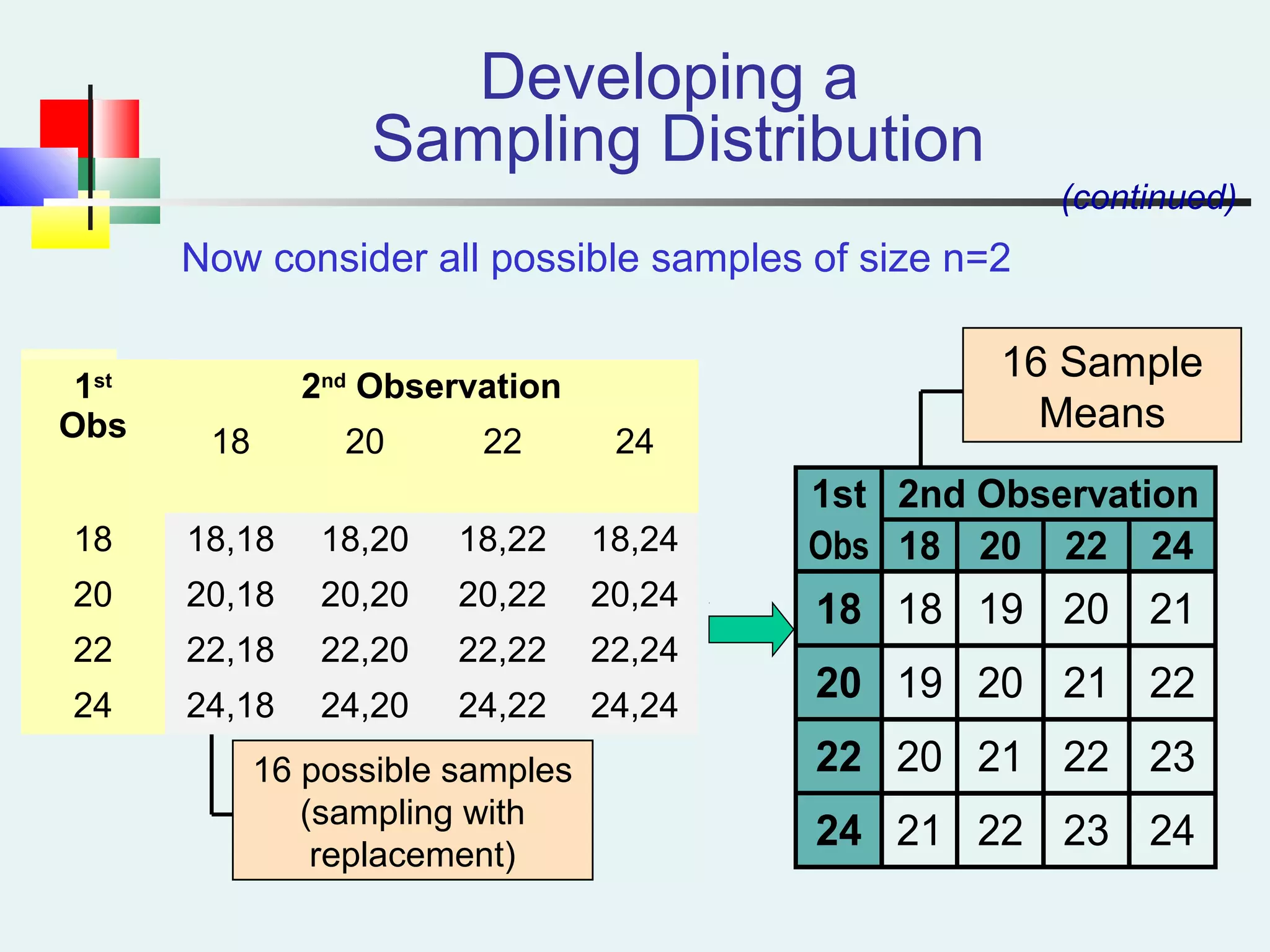
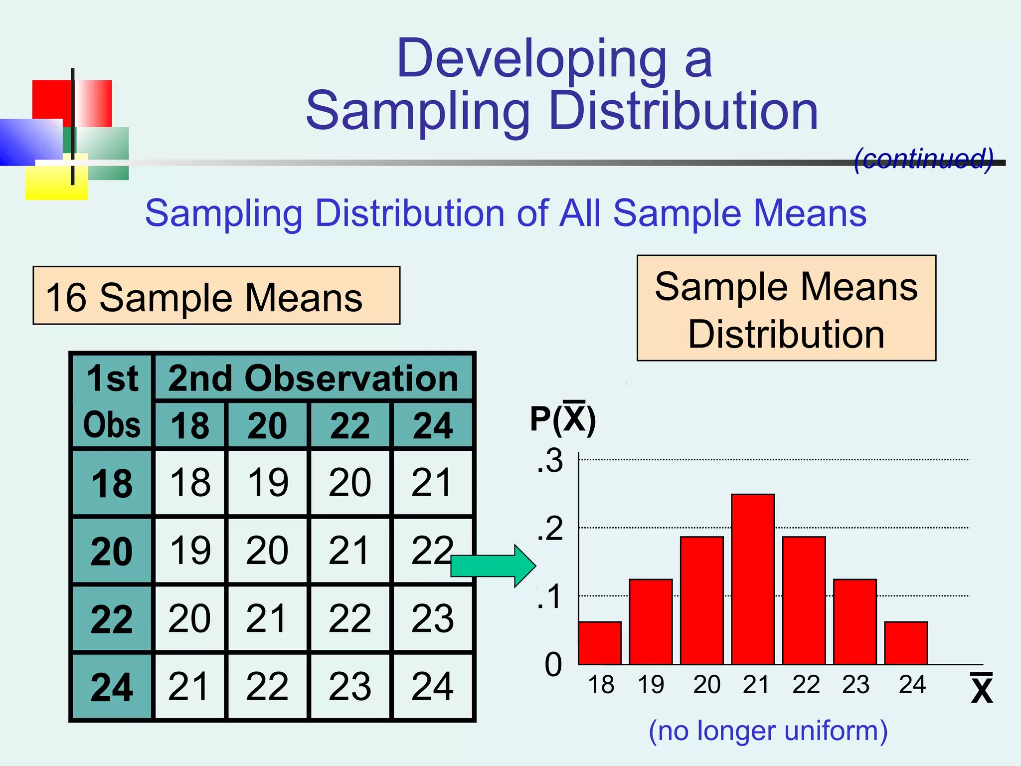
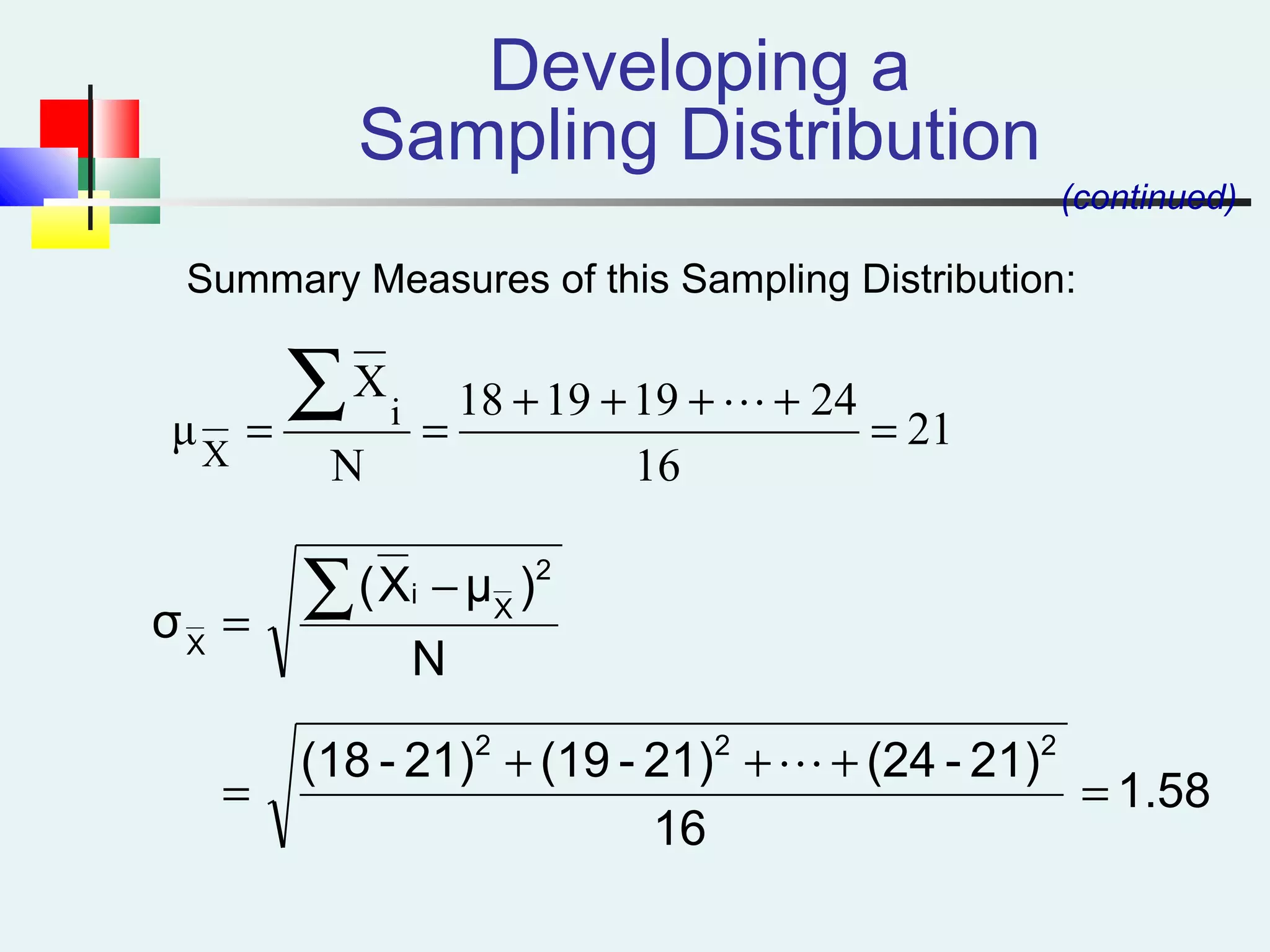
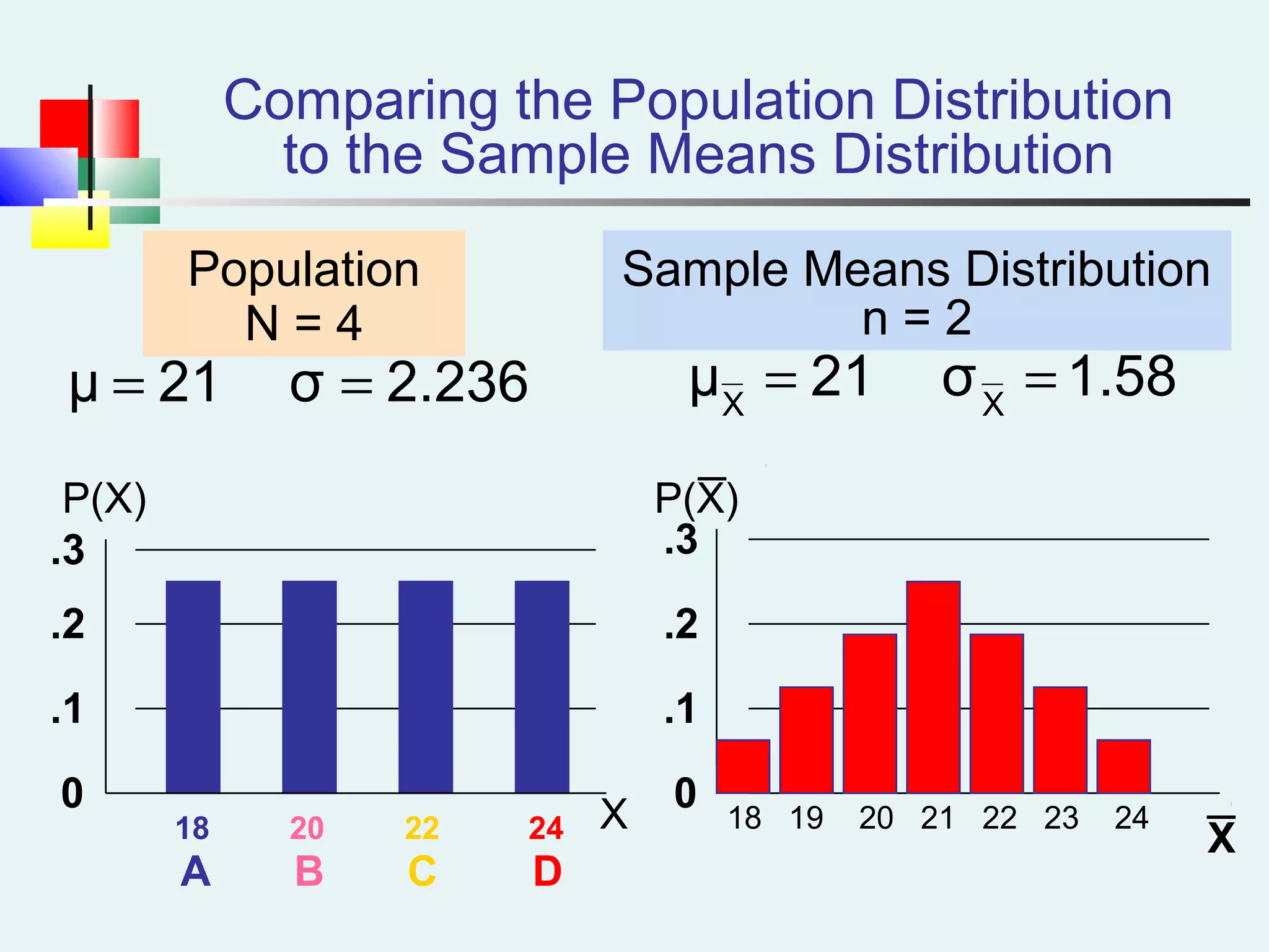
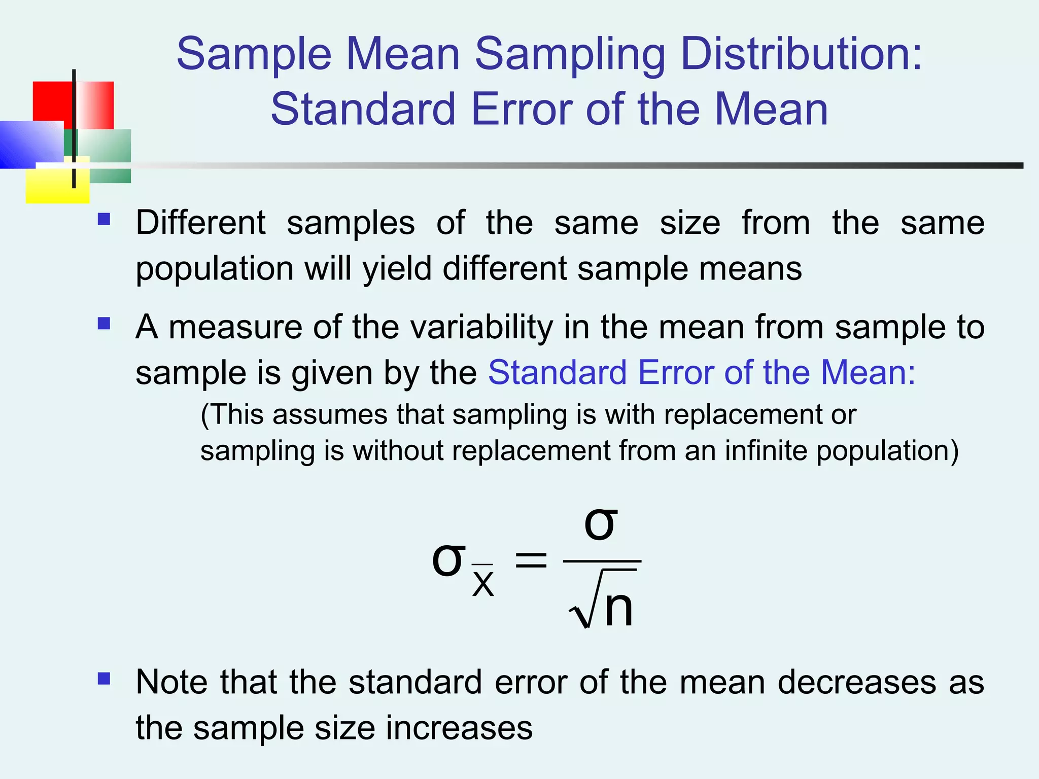
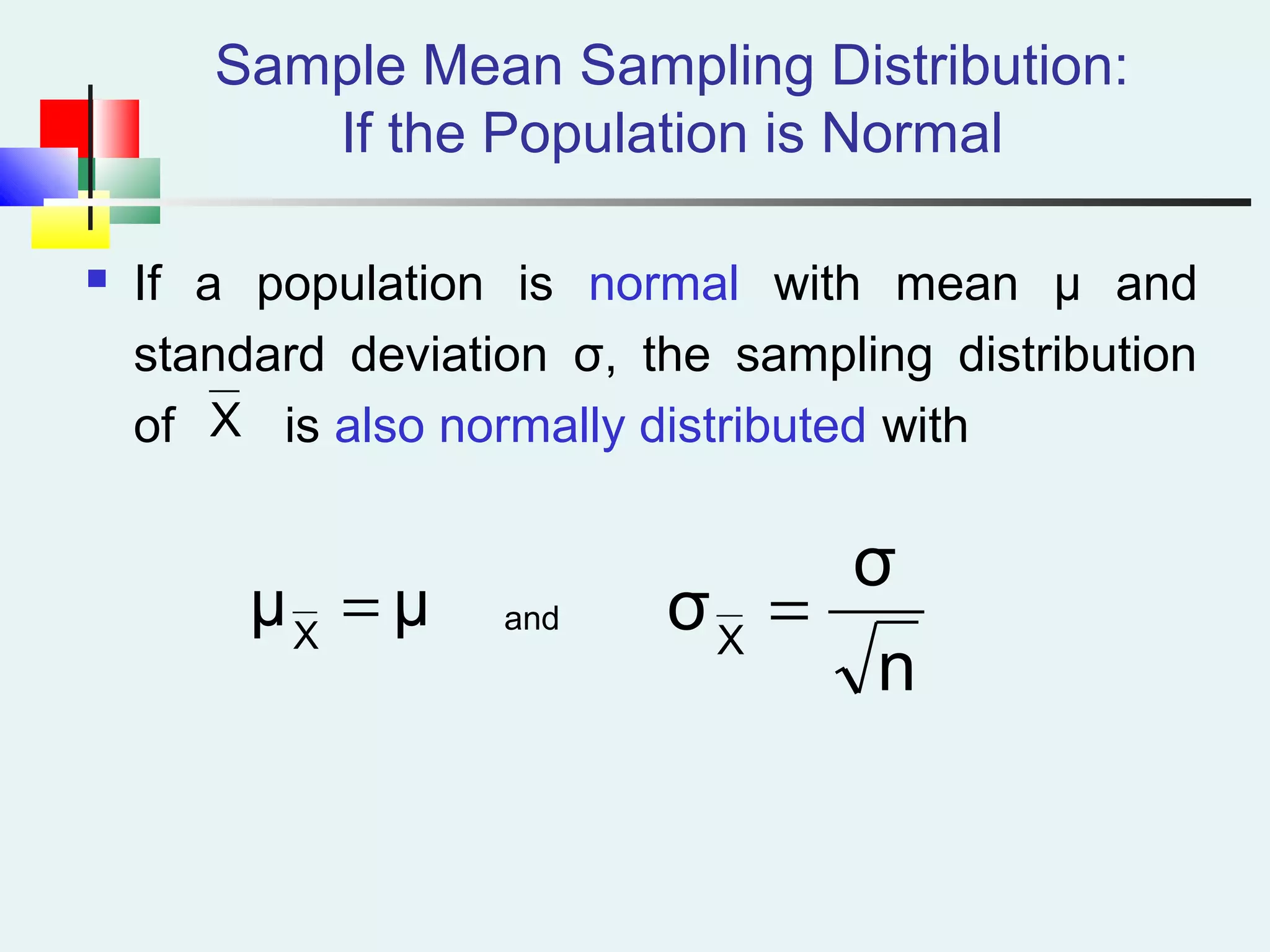
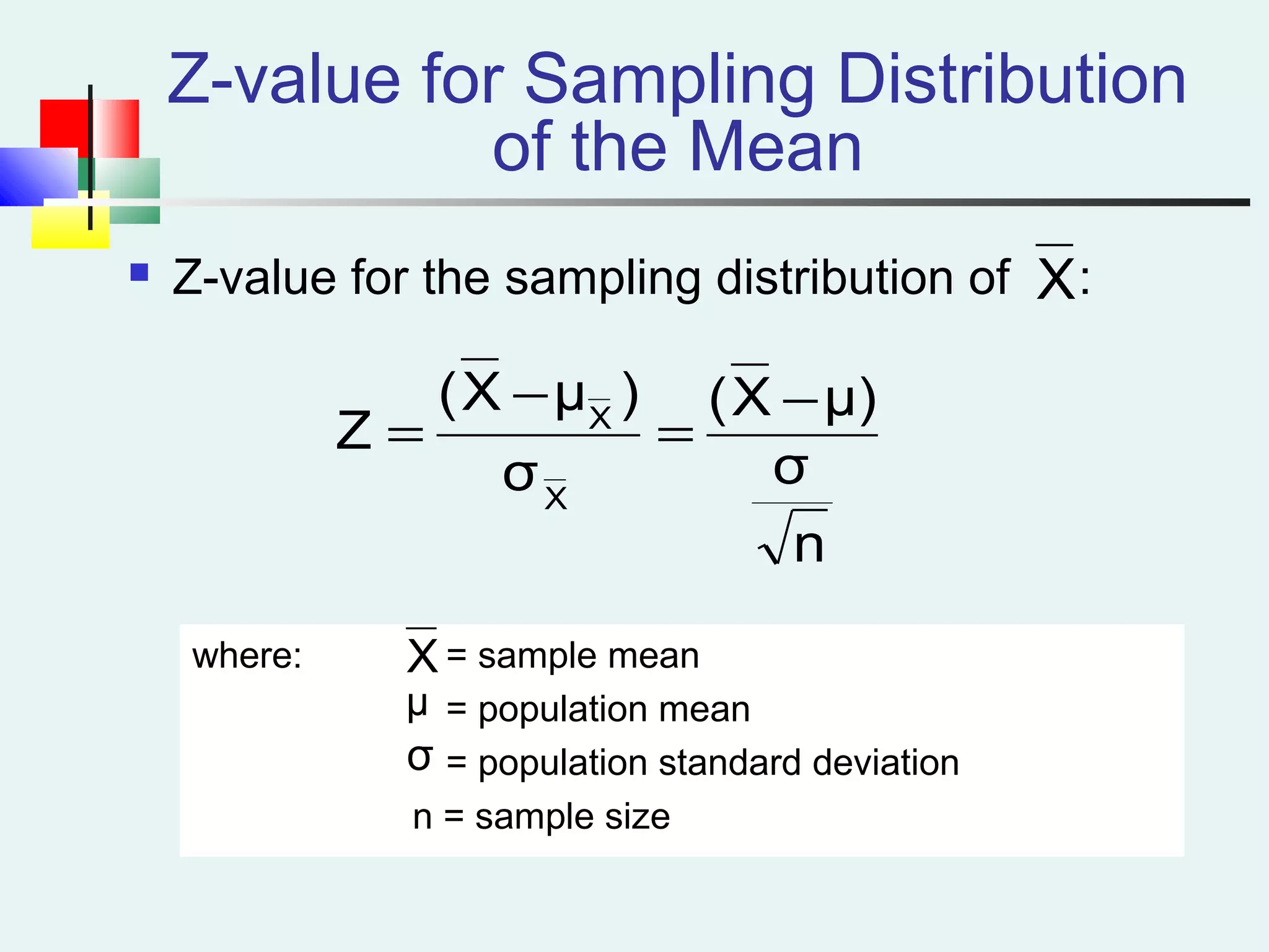
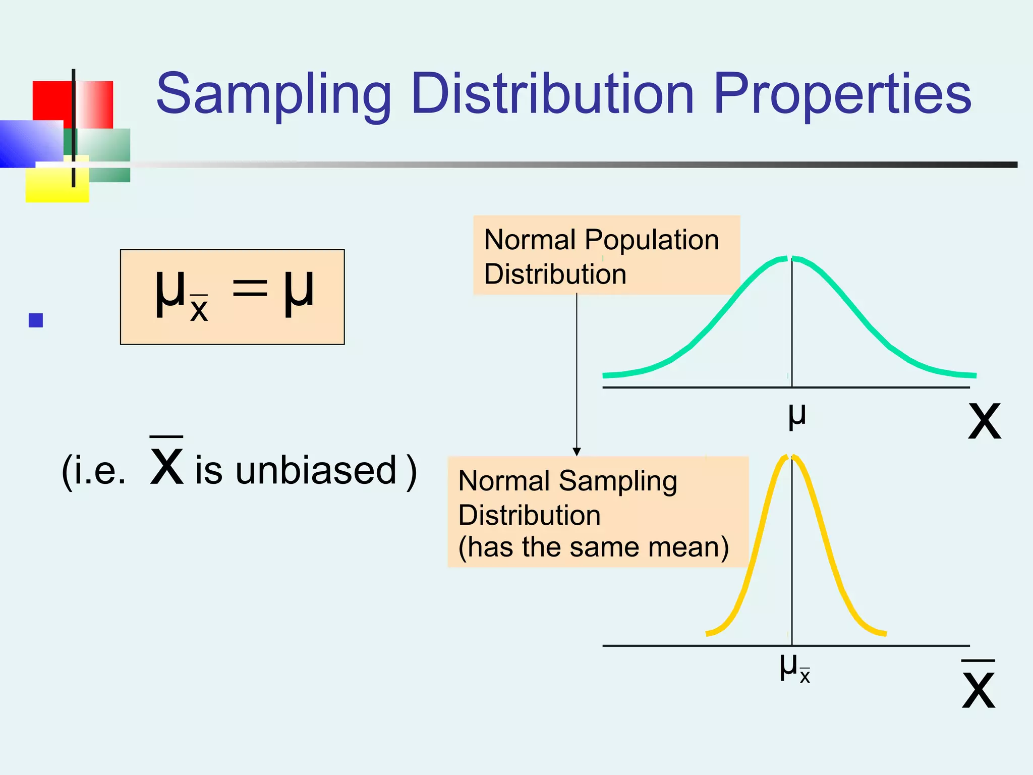
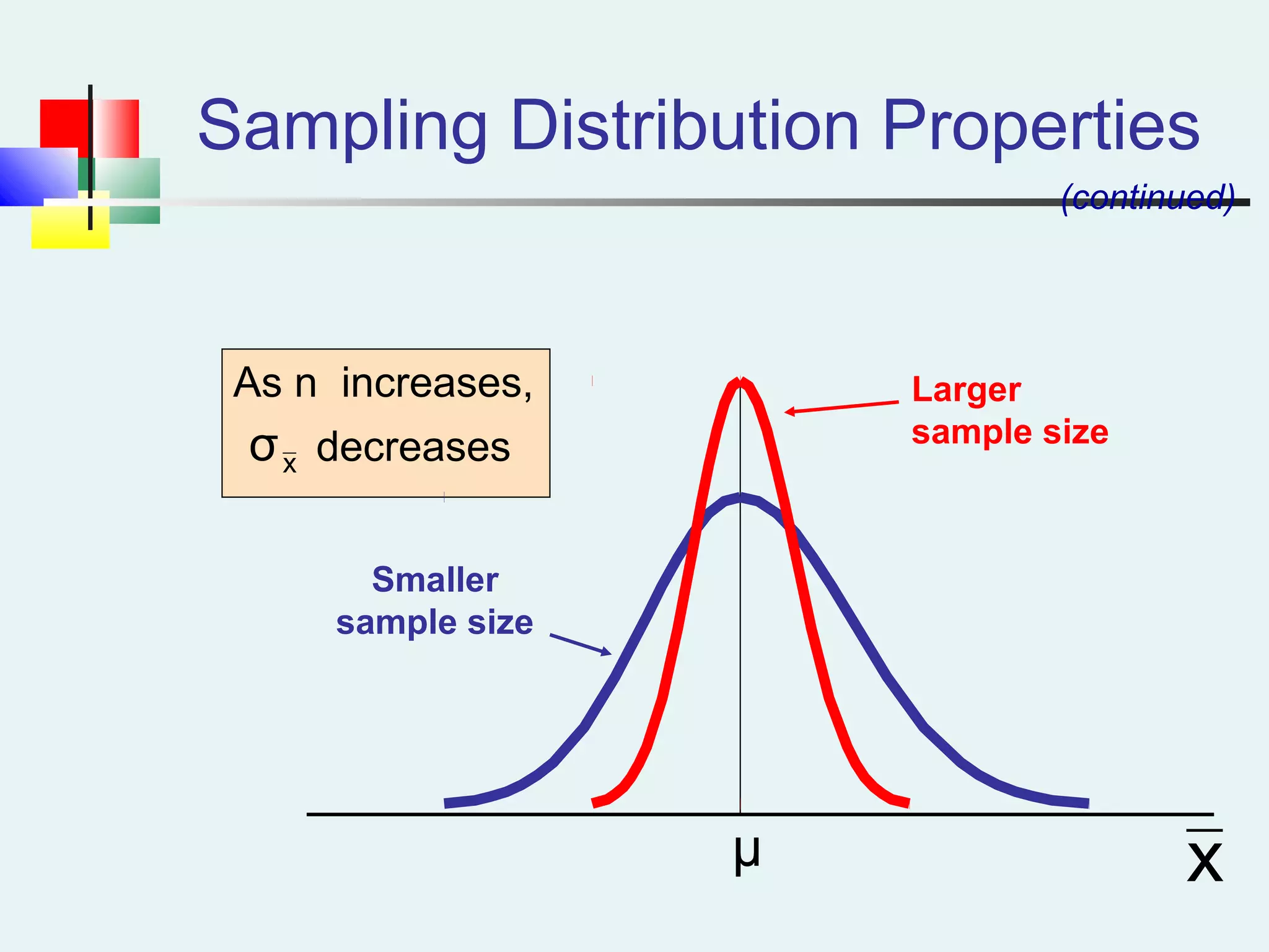
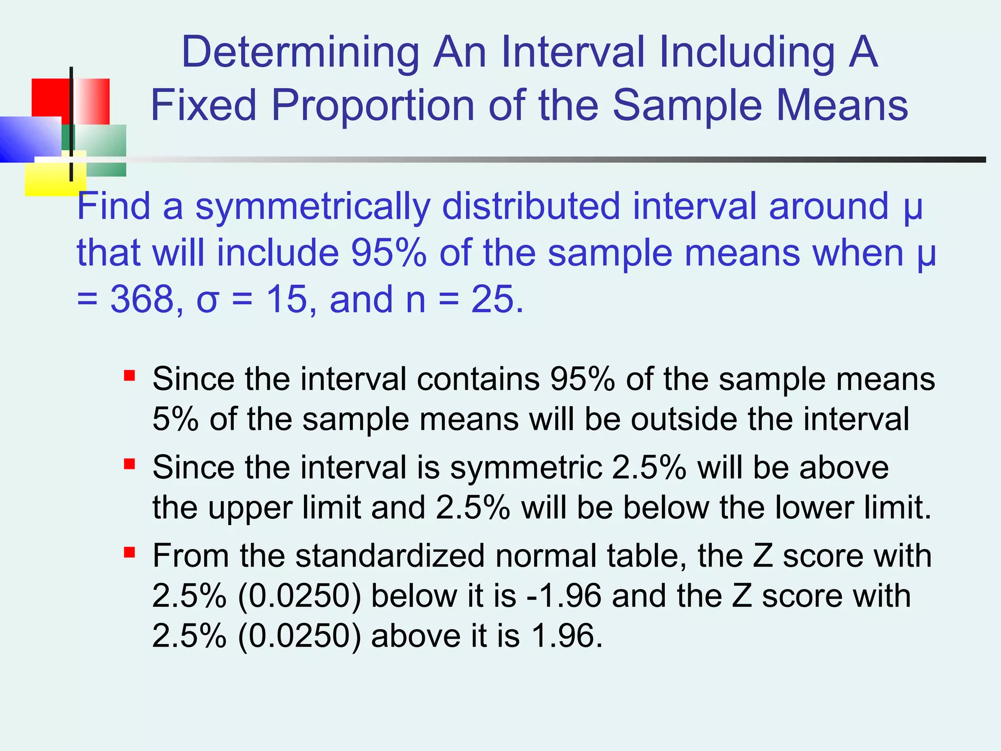
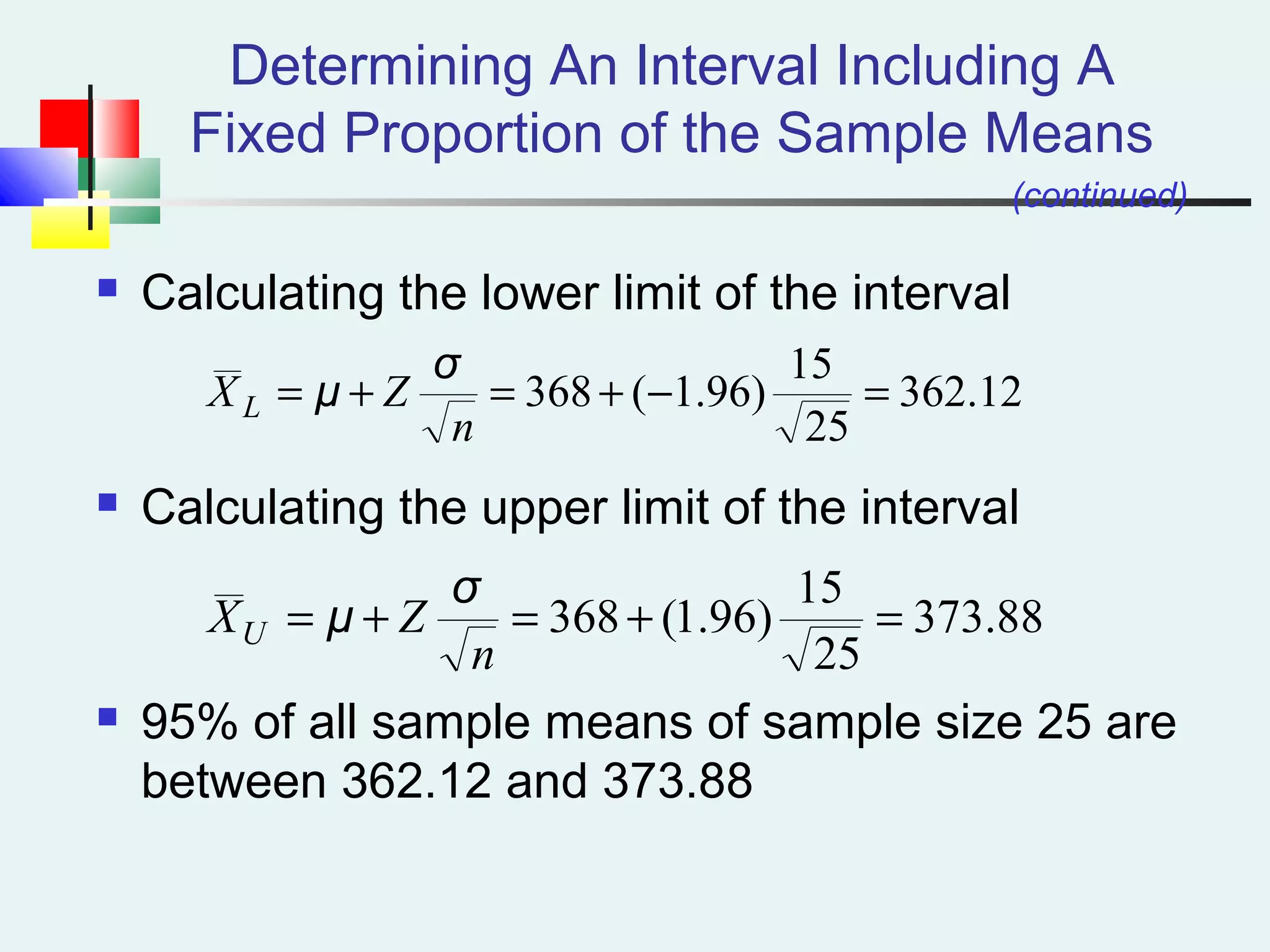
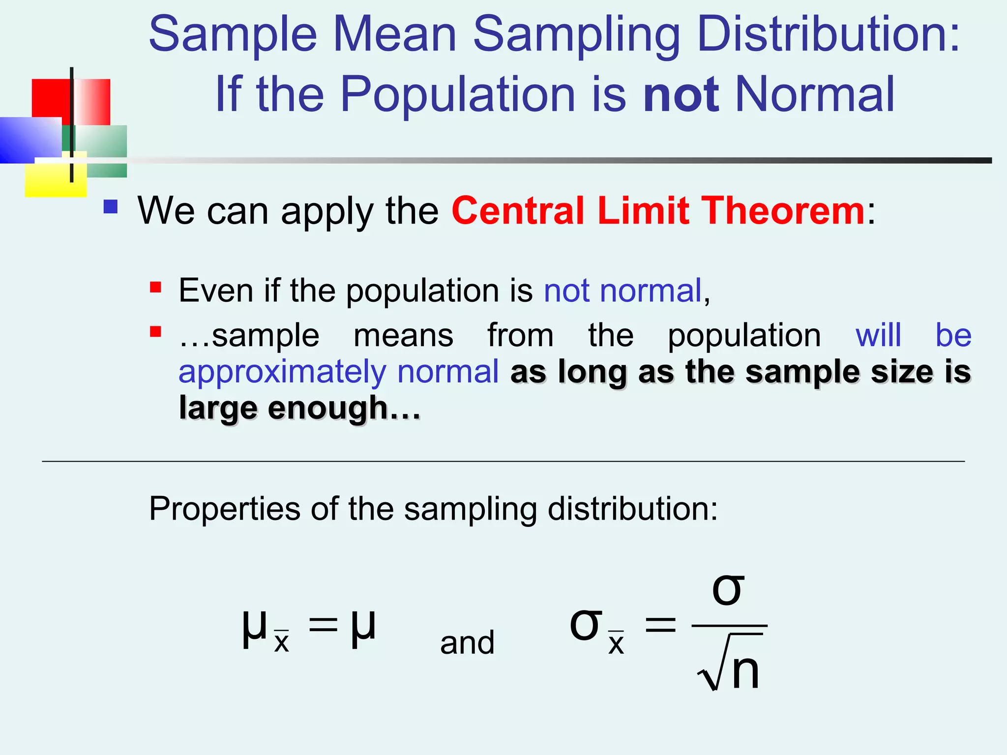
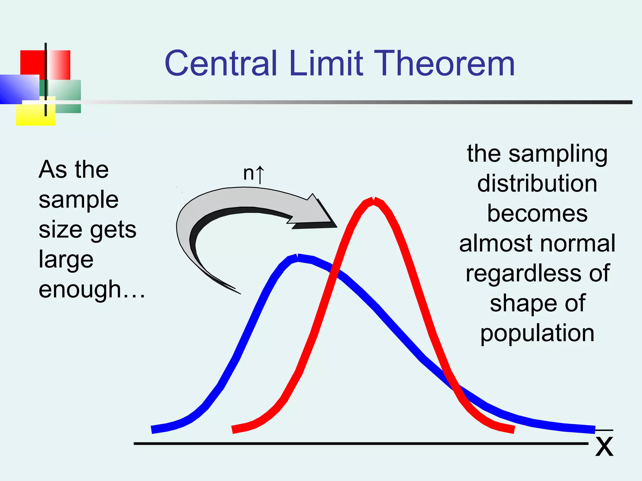
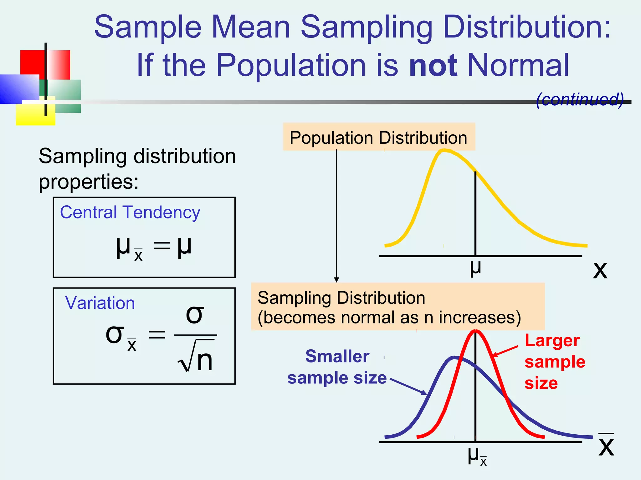
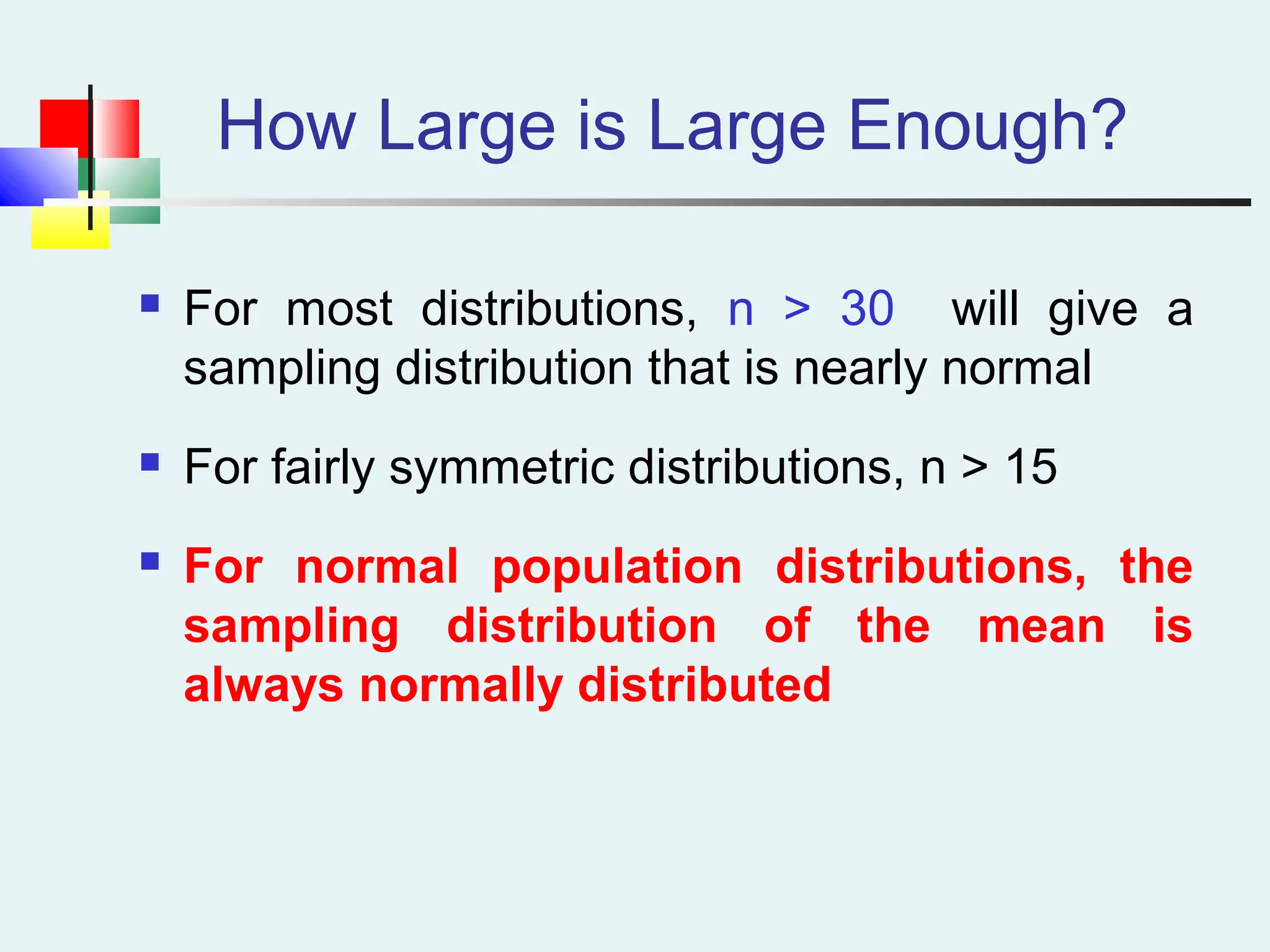
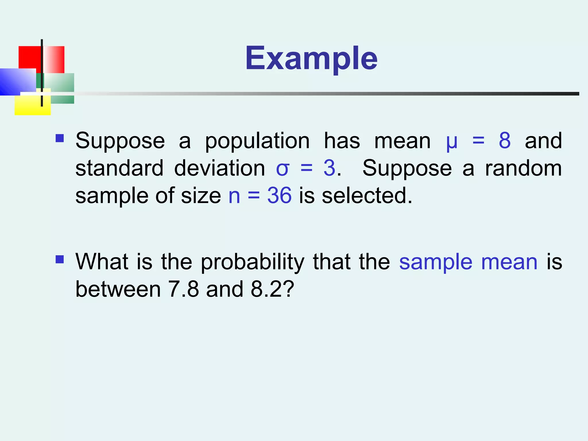
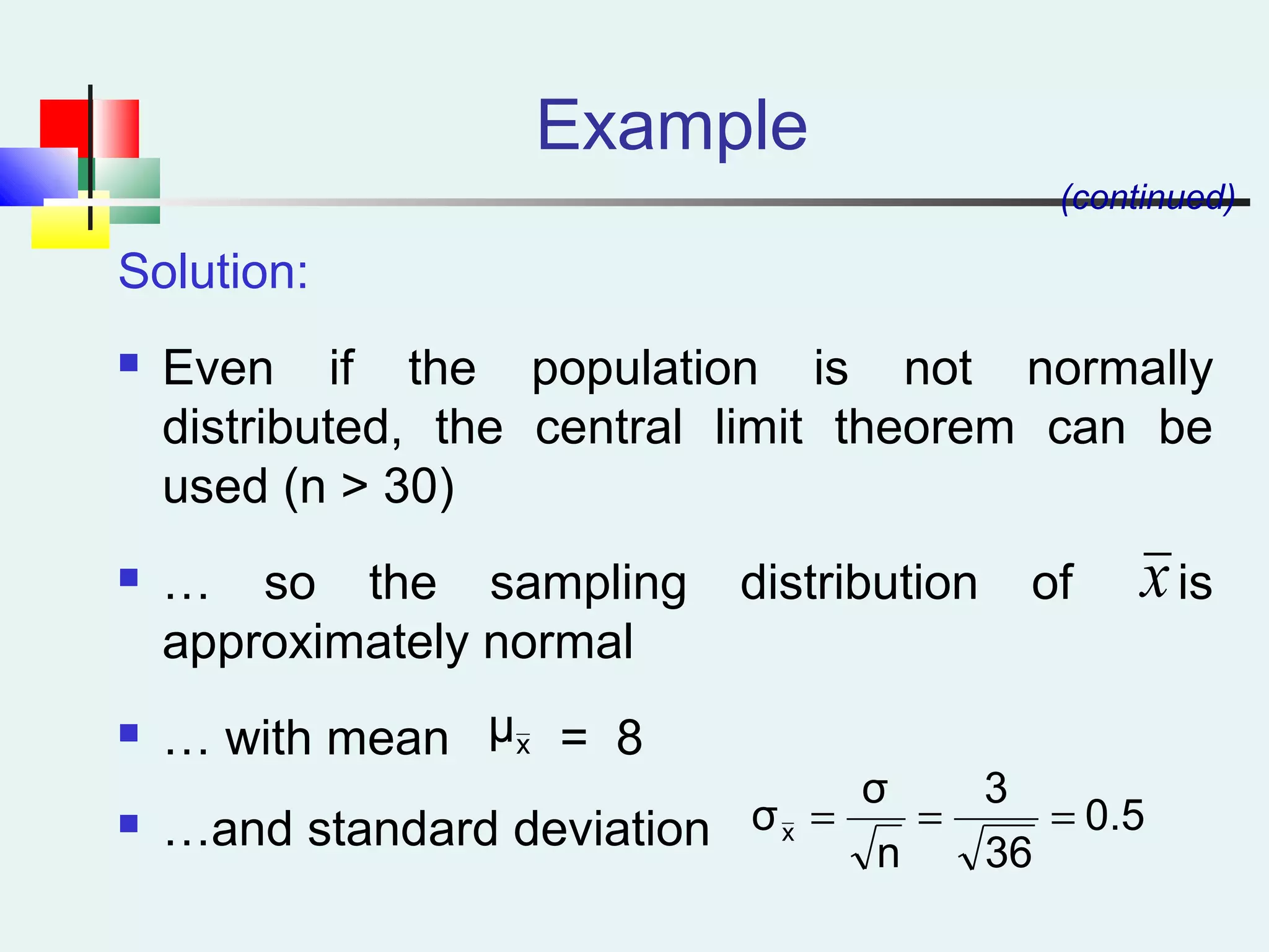
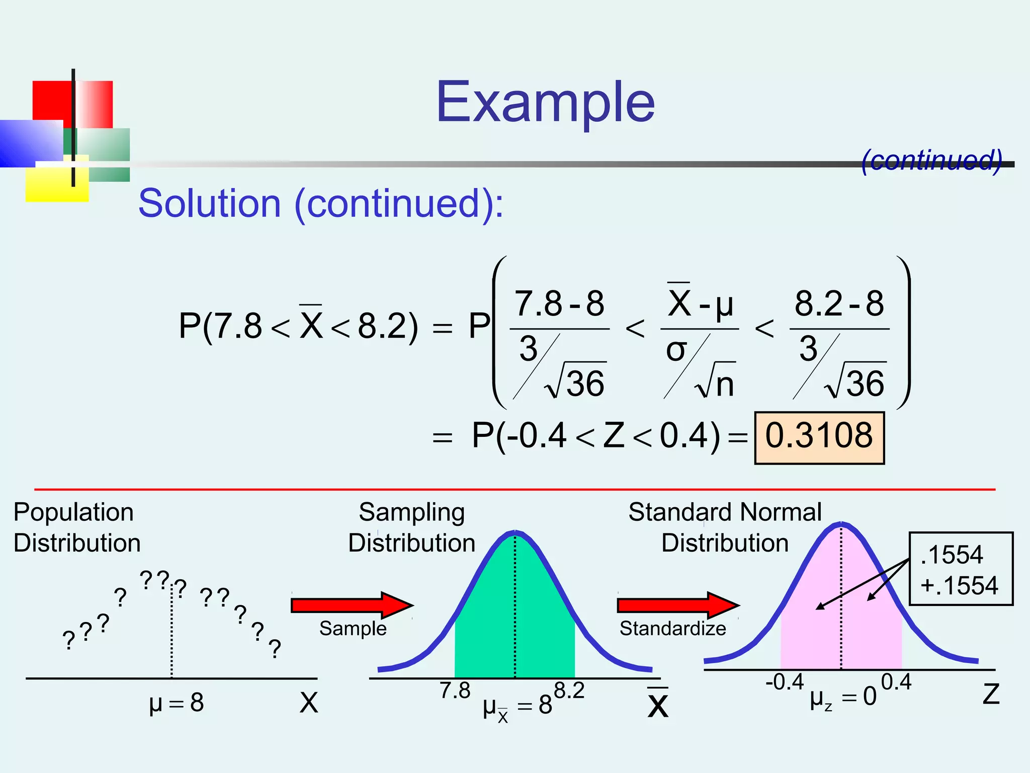
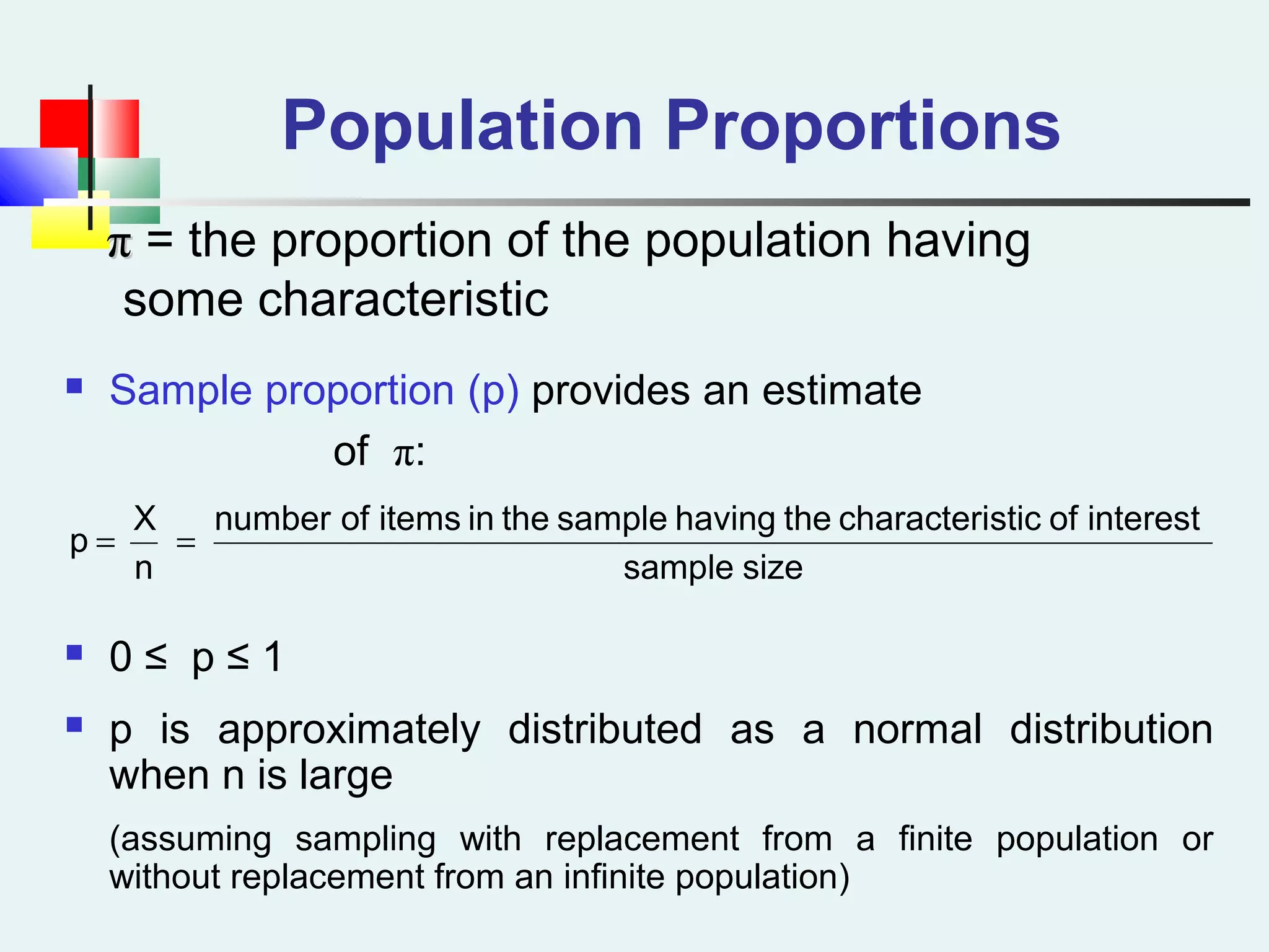
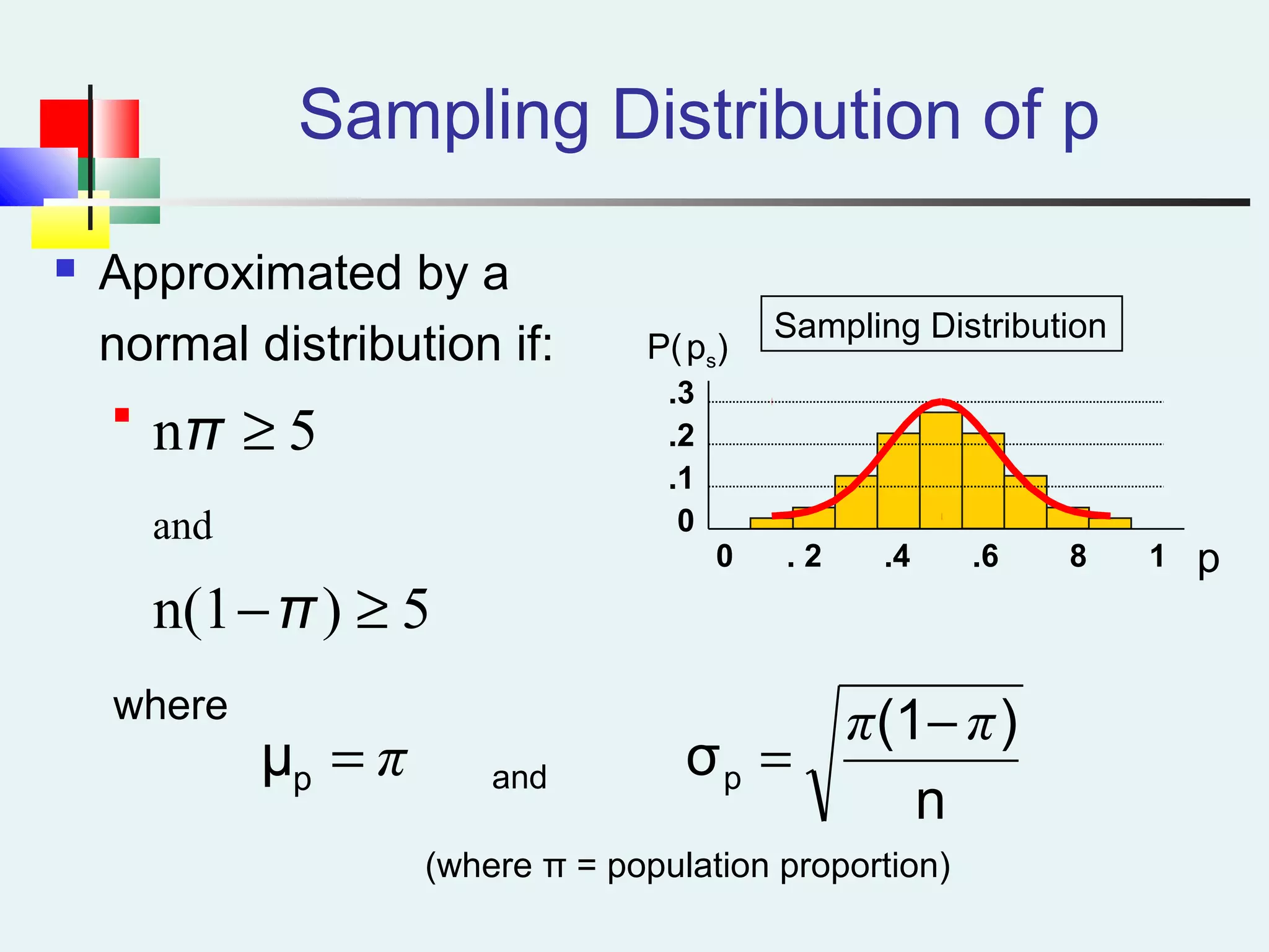
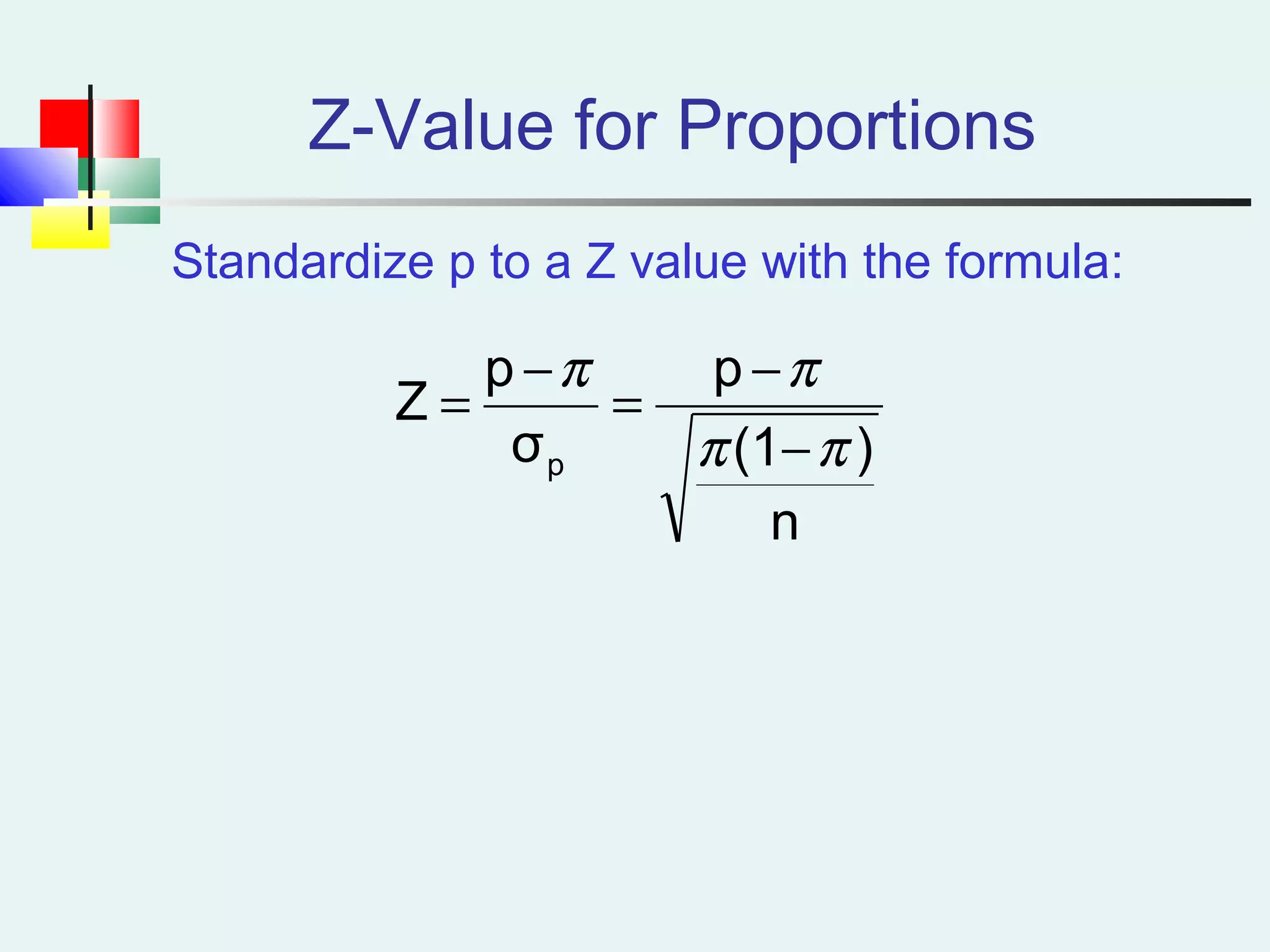
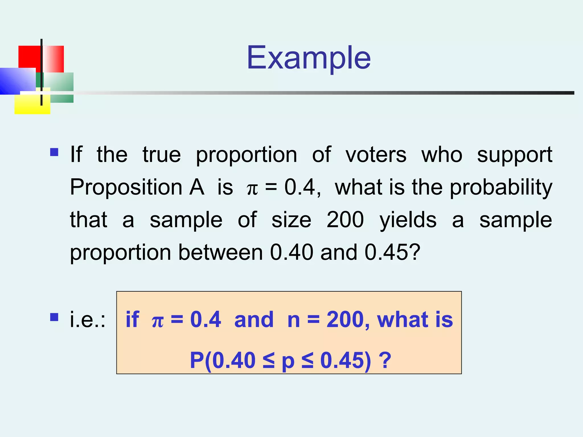
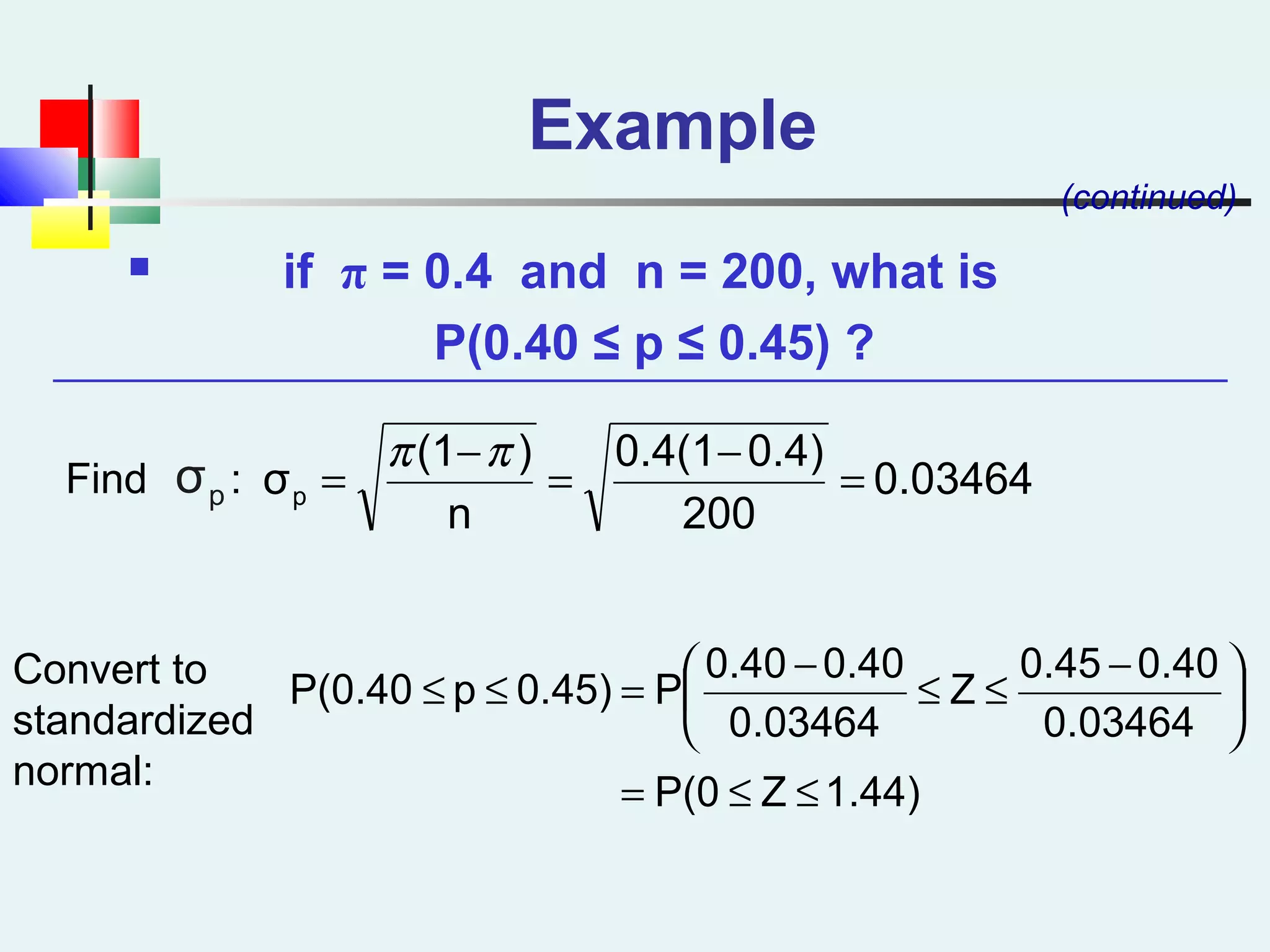
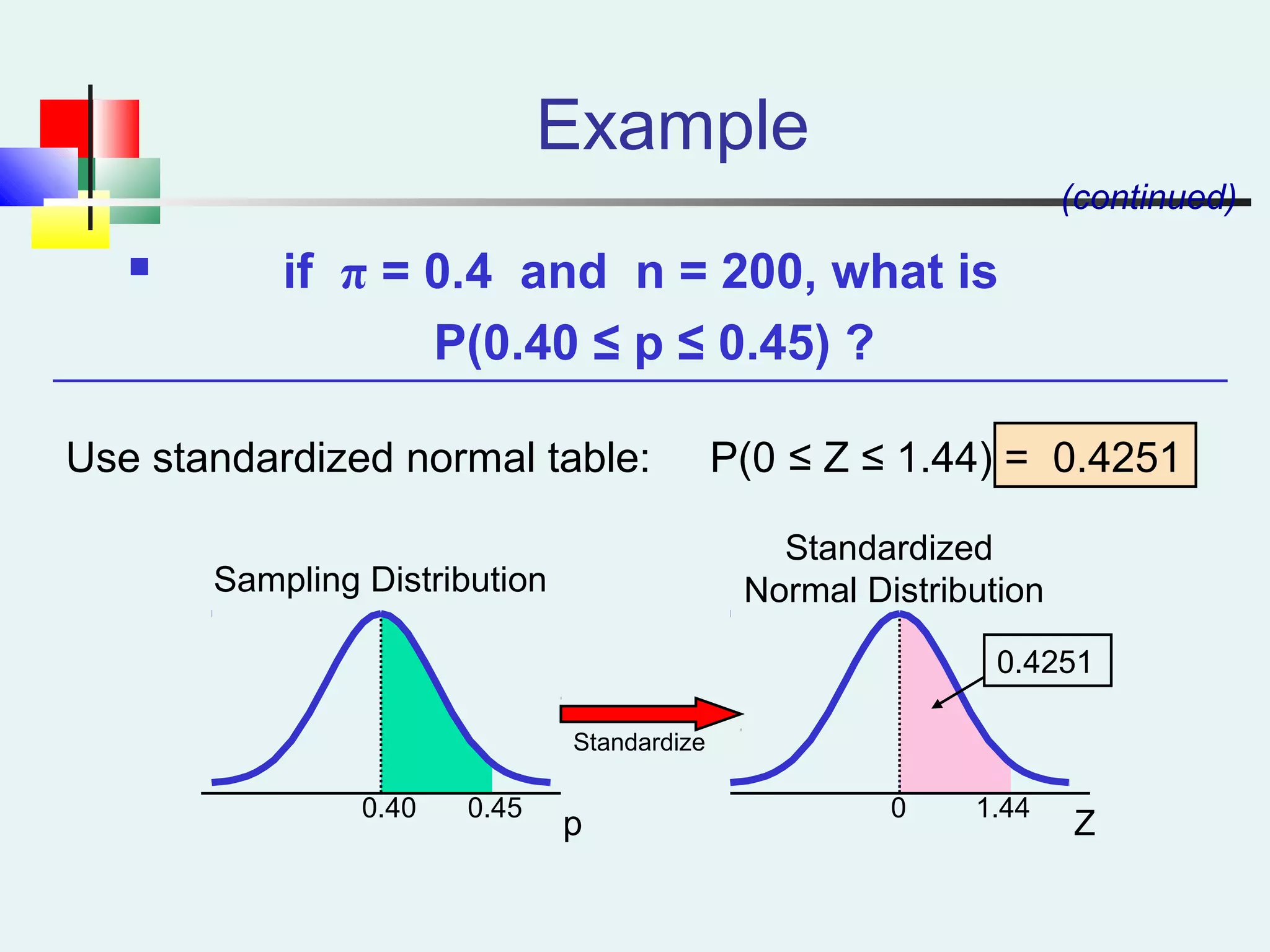
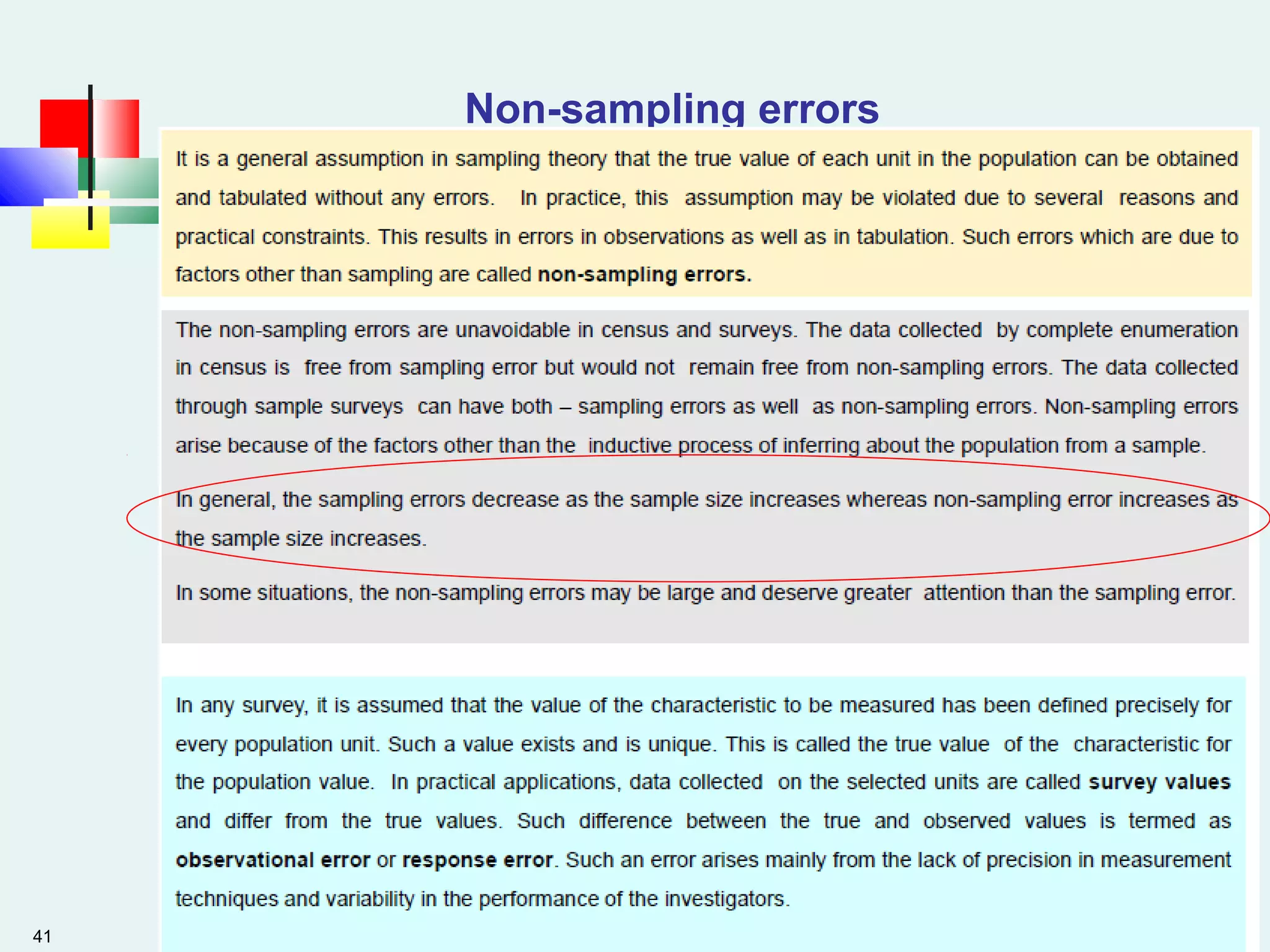
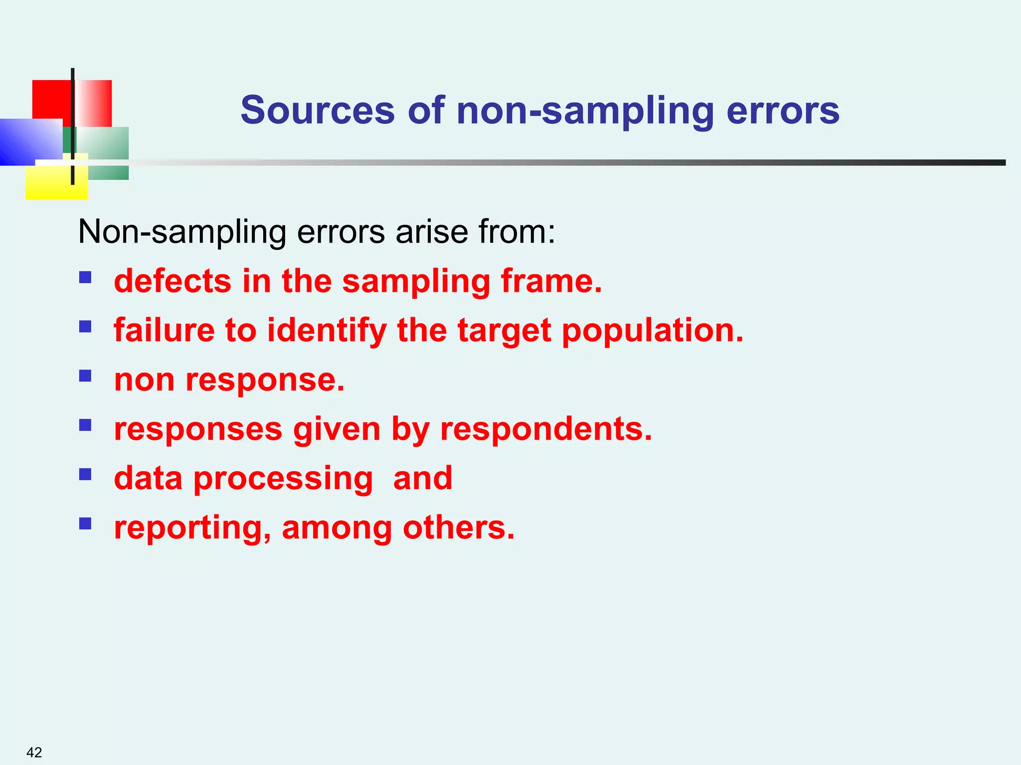
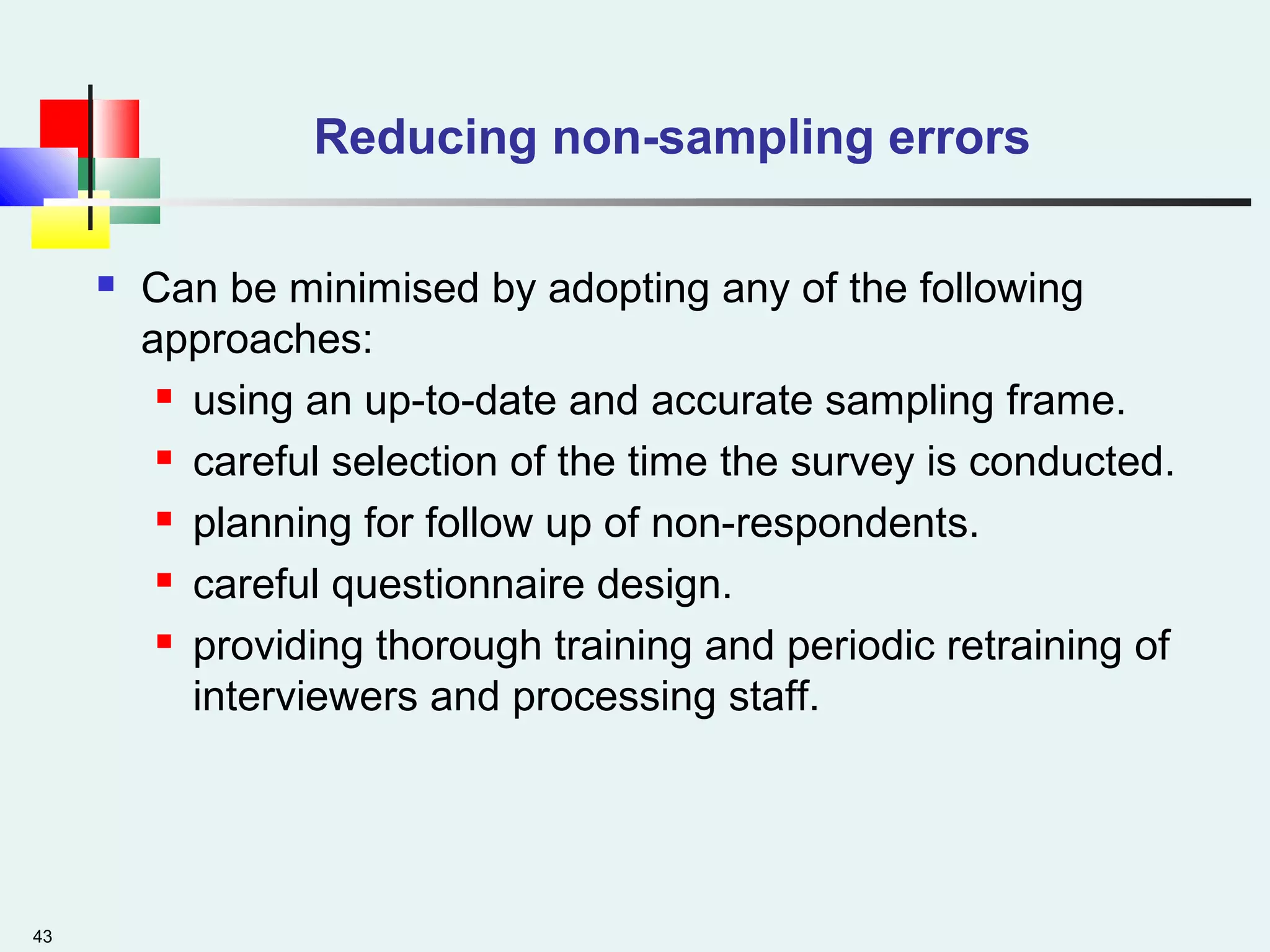
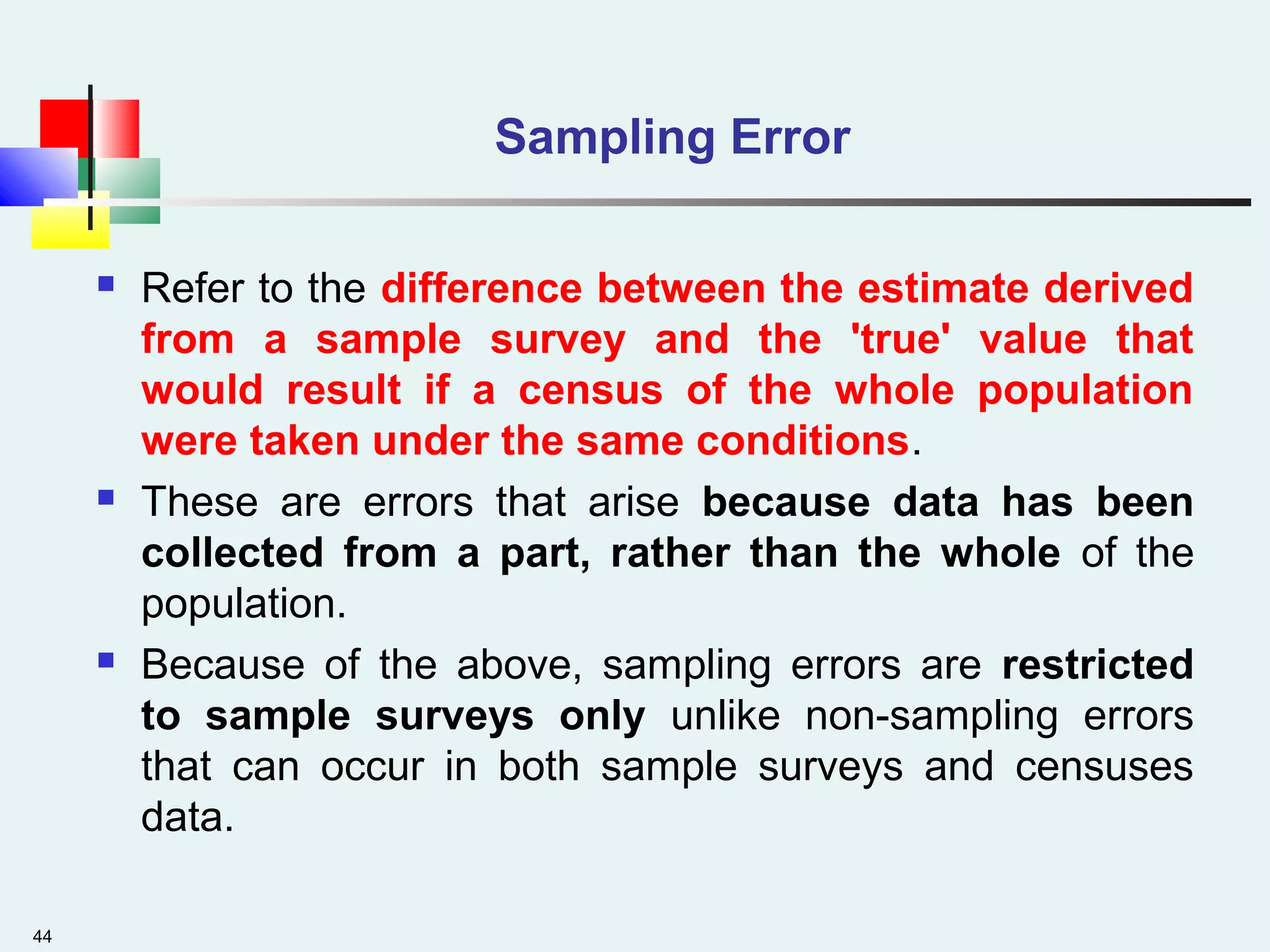
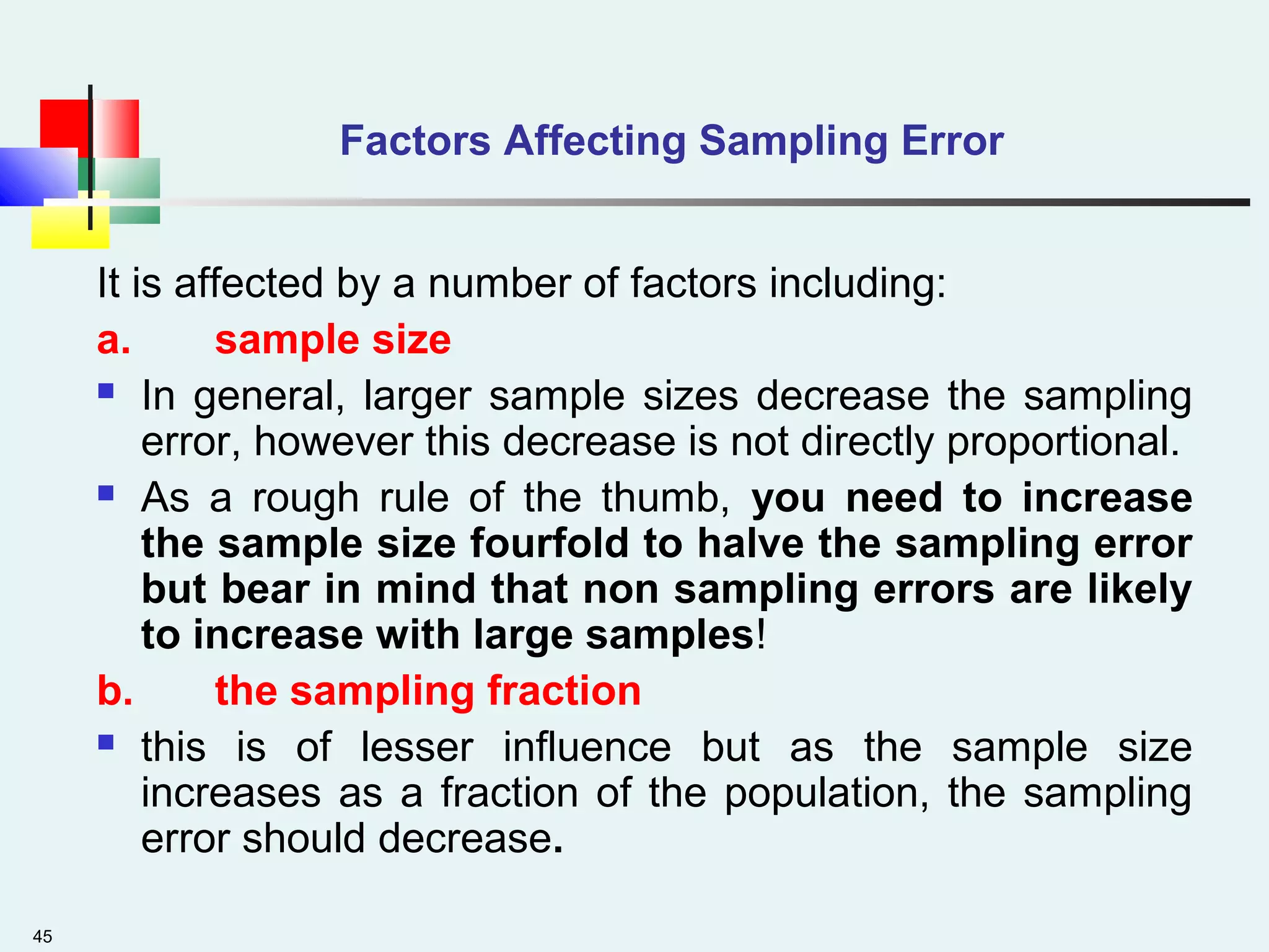
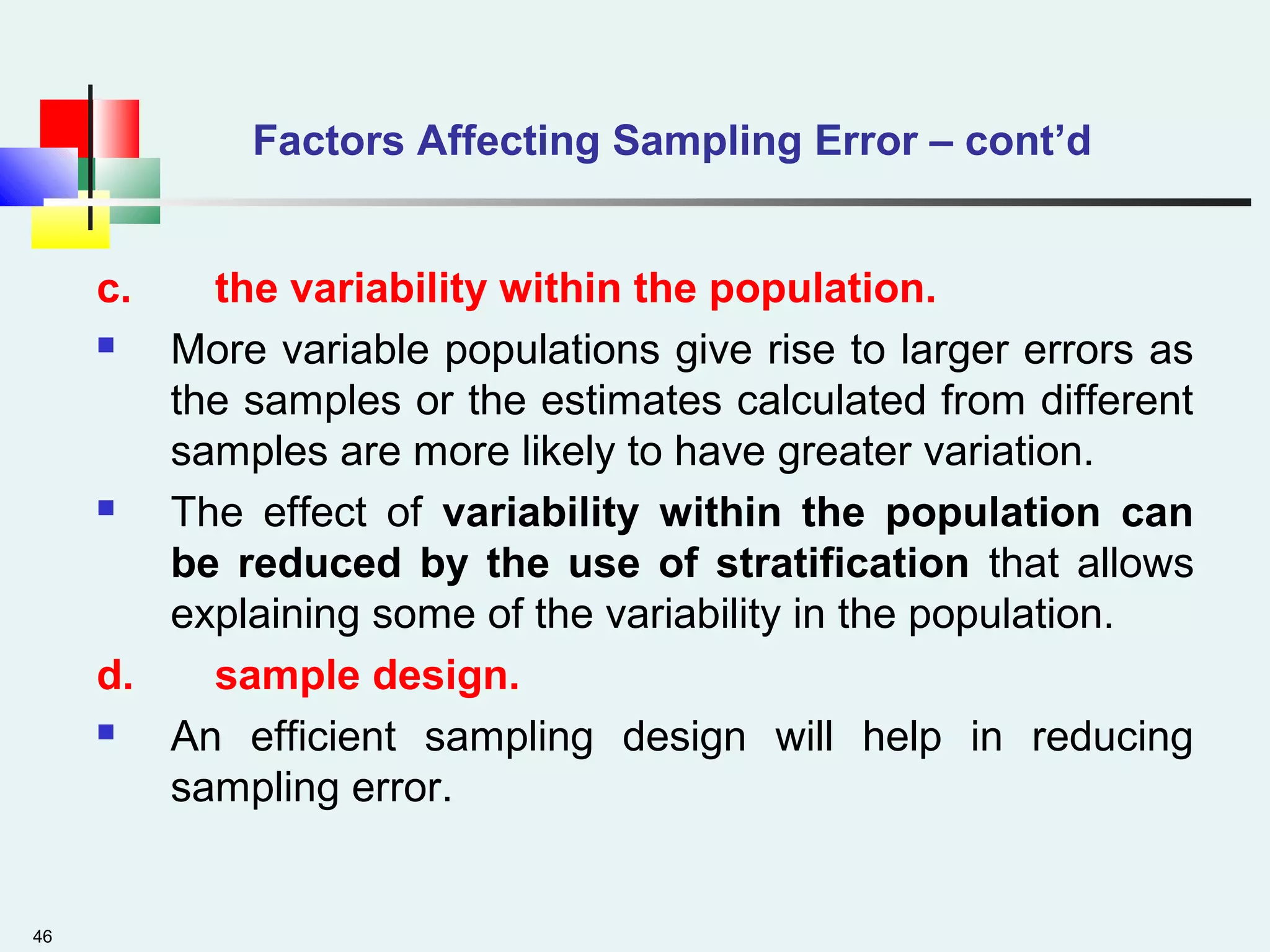
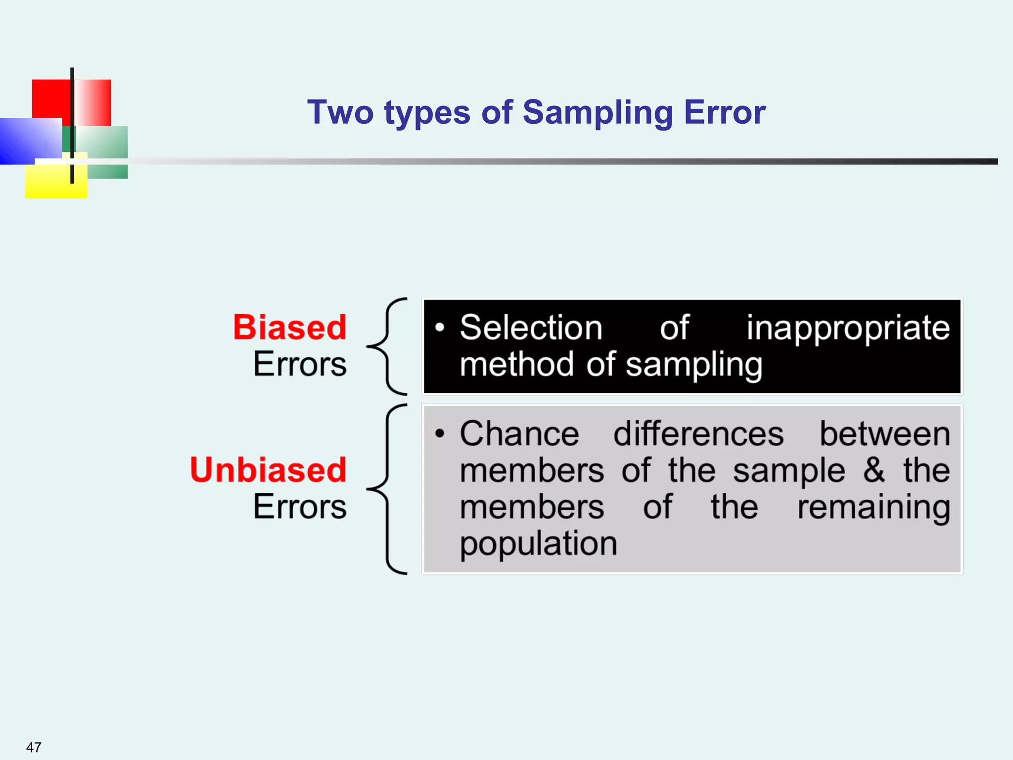
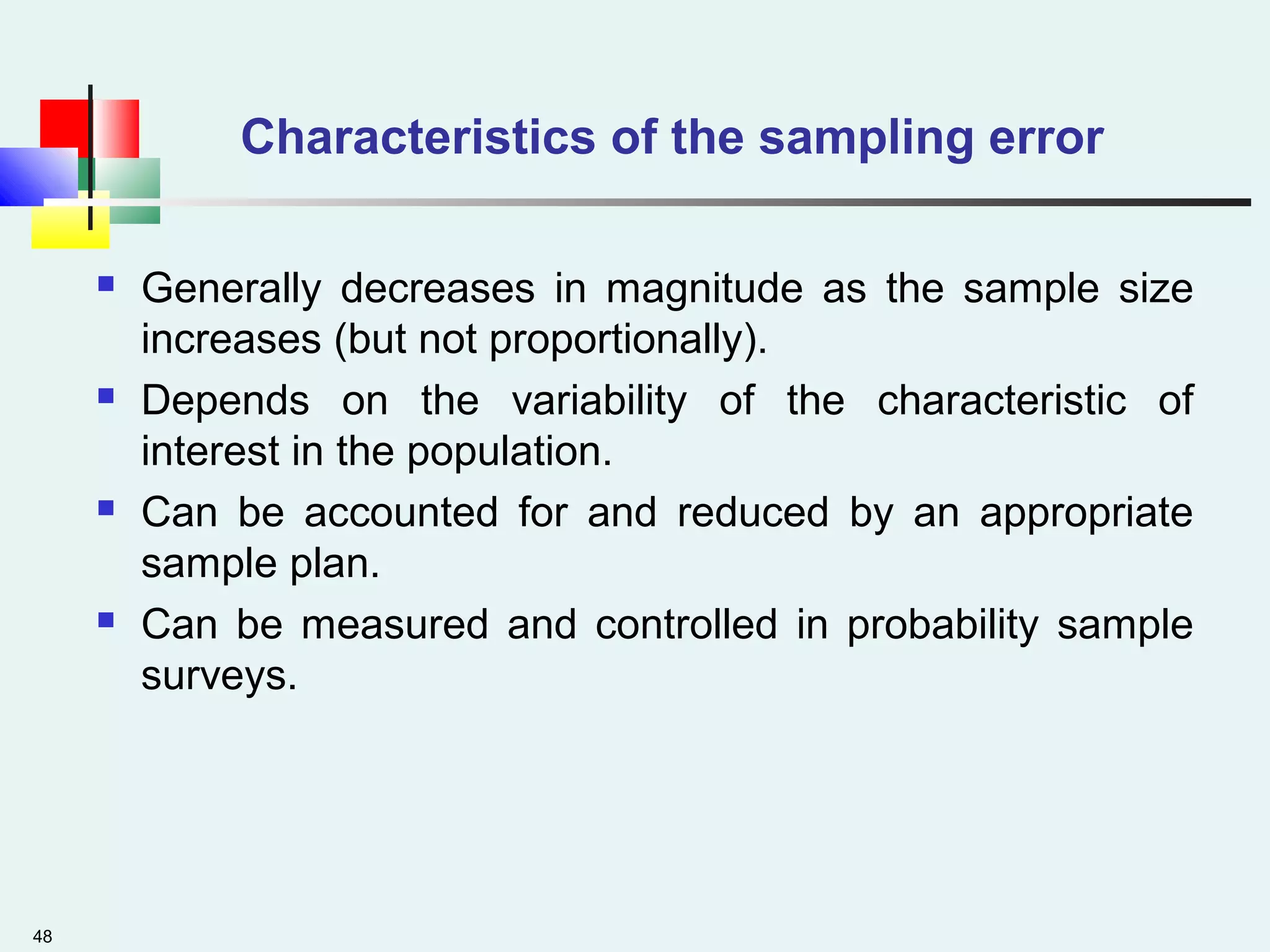
This document discusses sampling and sampling distributions. It begins by explaining why sampling is preferable to a census in terms of time, cost and practicality. It then defines the sampling frame as the listing of items that make up the population. Different types of samples are described, including probability and non-probability samples. Probability samples include simple random, systematic, stratified, and cluster samples. Key aspects of each type are defined. The document also discusses sampling distributions and how the distribution of sample statistics such as means and proportions can be approximated as normal even if the population is not normal, due to the central limit theorem. It provides examples of how to calculate probabilities and intervals for sampling distributions.

1. SamplingSampling and Sampling Distributions

2. Why Sample?
 Selecting a sample is less time-consuming than
selecting every item in the population (census).
 Selecting a sample is less costly than selecting
every item in the population.
 An analysis of a sample is less cumbersome
and more practical than an analysis of the
entire population.

3. A Sampling Process Begins With A
Sampling Frame
 The sampling frame is a listing of items that
make up the population
 Frames are data sources such as population
lists, directories, or maps
 Inaccurate or biased results can result if a
frame excludes certain portions of the
population
 Using different frames to generate data can
lead to dissimilar conclusions

4. Types of Samples
Samples
Non-Probability
Samples
Judgment
Probability Samples
Simple
Random
Systematic
Stratified
Cluster
Convenience

5. Types of Samples:
Nonprobability Sample
 In a nonprobability sample, items included are
chosen without regard to their probability of
occurrence.
 In convenience sampling, items are selected based
only on the fact that they are easy, inexpensive, or
convenient to sample.
 In a judgment sample, you get the opinions of pre-
selected experts in the subject matter.

6. Types of Samples:
Probability Sample
 In a probability sample, items in the
sample are chosen on the basis of known
probabilities.
Probability Samples
Simple
Random Systematic Stratified Cluster

7. Probability Sample:
Simple Random Sample
 Every individual or item from the frame has an
equal chance of being selected
 Selection may be with replacement (selected
individual is returned to frame for possible
reselection) or without replacement (selected
individual isn’t returned to the frame).
 Samples obtained from table of random
numbers or computer random number
generators.

8.  Decide on sample size: n
 Divide frame of N individuals into groups of k
individuals: k=N/n
 Randomly select one individual from the 1st
group
 Select every kth
individual thereafter
Probability Sample:
Systematic Sample
N = 40
n = 4
k = 10
First Group

9. Probability Sample:
Stratified Sample
 Divide population into two or more subgroups (called strata)
according to some common characteristic
 A simple random sample is selected from each subgroup, with
sample sizes proportional to strata sizes
 Samples from subgroups are combined into one
 This is a common technique when sampling population of voters,
stratifying across racial or socio-economic lines.
Population
Divided
into 4
strata

10. Probability Sample
Cluster Sample
 Population is divided into several “clusters,” each representative of
the population
 A simple random sample of clusters is selected
 All items in the selected clusters can be used, or items can be
chosen from a cluster using another probability sampling technique
 A common application of cluster sampling involves election exit polls,
where certain election districts are selected and sampled.
Population
divided into
16 clusters. Randomly selected
clusters for sample

11. Probability Sample:
Comparing Sampling Methods
 Simple random sample and Systematic sample
 Simple to use
 May not be a good representation of the population’s
underlying characteristics
 Stratified sample
 Ensures representation of individuals across the entire
population
 Cluster sample
 More cost effective
 Less efficient (need larger sample to acquire the same
level of precision)

12. Sampling Distributions
 A sampling distribution is a distribution of all of the
possible values of a sample statistic for a given size
sample selected from a population.
 For example, suppose you sample 50 students from your
college regarding their mean CGPA. If you obtained
many different samples of 50, you will compute a
different mean for each sample. We are interested in the
distribution of all potential mean CGPA we might
calculate for any given sample of 50 students.

13. Developing a
Sampling Distribution
 Assume there is a population …
 Population size N=4
 Random variable, X,
is age of individuals
 Values of X: 18, 20,
22, 24 (years)
A B C D

14. .3
.2
.1
0
18 20 22 24
A B C D
Uniform Distribution
P(x)
x
(continued)
Summary Measures for the Population Distribution:
Developing a
Sampling Distribution
21
4
24222018
N
X
μ i
=
+++
=
=
∑
2.236
N
μ)(X
σ
2
i
=
−
=
∑

15. 16 possible samples
(sampling with
replacement)
Now consider all possible samples of size n=2
1st 2nd Observation
Obs 18 20 22 24
18 18 19 20 21
20 19 20 21 22
22 20 21 22 23
24 21 22 23 24
(continued)
Developing a
Sampling Distribution
16 Sample
Means
1st
Obs
2nd
Observation
18 20 22 24
18 18,18 18,20 18,22 18,24
20 20,18 20,20 20,22 20,24
22 22,18 22,20 22,22 22,24
24 24,18 24,20 24,22 24,24

16. 1st 2nd Observation
Obs 18 20 22 24
18 18 19 20 21
20 19 20 21 22
22 20 21 22 23
24 21 22 23 24
Sampling Distribution of All Sample Means
18 19 20 21 22 23 24
0
.1
.2
.3
P(X)
X
Sample Means
Distribution
16 Sample Means
_
Developing a
Sampling Distribution
(continued)
(no longer uniform)
_

17. Summary Measures of this Sampling Distribution:
Developing a
Sampling Distribution
(continued)
21
16
24191918
N
X
μ i
X
=
++++
==
∑ 
1.58
16
21)-(2421)-(1921)-(18
N
)μX(
σ
222
2
X
i
X
=
+++
=
−
=
∑


18. Comparing the Population Distribution
to the Sample Means Distribution
18 19 20 21 22 23 24
0
.1
.2
.3
P(X)
X18 20 22 24
A B C D
0
.1
.2
.3
Population
N = 4
P(X)
X _
1.58σ21μ XX
==2.236σ21μ ==
Sample Means Distribution
n = 2
_

19. Sample Mean Sampling Distribution:
Standard Error of the Mean
 Different samples of the same size from the same
population will yield different sample means
 A measure of the variability in the mean from sample to
sample is given by the Standard Error of the Mean:
(This assumes that sampling is with replacement or
sampling is without replacement from an infinite population)
 Note that the standard error of the mean decreases as
the sample size increases
n
σ
σX
=

20. Sample Mean Sampling Distribution:
If the Population is Normal
 If a population is normal with mean μ and
standard deviation σ, the sampling distribution
of is also normally distributed with
and
X
μμX
=
n
σ
σX
=

21. Z-value for Sampling Distribution
of the Mean
 Z-value for the sampling distribution of :
where: = sample mean
= population mean
= population standard deviation
n = sample size
X
μ
σ
n
σ
μ)X(
σ
)μX(
Z
X
X −
=
−
=
X

22. Normal Population
Distribution
Normal Sampling
Distribution
(has the same mean)
Sampling Distribution Properties

(i.e. is unbiased )x
x
x
μμx =
μ
xμ

23. Sampling Distribution Properties
As n increases,
decreases
Larger
sample size
Smaller
sample size
x
(continued)
xσ
μ

24. Determining An Interval Including A
Fixed Proportion of the Sample Means
Find a symmetrically distributed interval around µ
that will include 95% of the sample means when µ
= 368, σ = 15, and n = 25.
 Since the interval contains 95% of the sample means
5% of the sample means will be outside the interval
 Since the interval is symmetric 2.5% will be above
the upper limit and 2.5% will be below the lower limit.
 From the standardized normal table, the Z score with
2.5% (0.0250) below it is -1.96 and the Z score with
2.5% (0.0250) above it is 1.96.

25. Determining An Interval Including A
Fixed Proportion of the Sample Means
 Calculating the lower limit of the interval
 Calculating the upper limit of the interval
 95% of all sample means of sample size 25 are
between 362.12 and 373.88
12.362
25
15
)96.1(368 =−+=+=
n
ZX L
σ
μ
(continued)
88.373
25
15
)96.1(368 =+=+=
n
ZXU
σ
μ

26. Sample Mean Sampling Distribution:
If the Population is not Normal
 We can apply the Central Limit Theorem:
 Even if the population is not normal,
 …sample means from the population will be
approximately normal as long as the sample size isas long as the sample size is
large enough…large enough…
Properties of the sampling distribution:
andμμx =
n
σ
σx =

27. n↑
Central Limit Theorem
As the
sample
size gets
large
enough…
the sampling
distribution
becomes
almost normal
regardless of
shape of
population
x

28. Population Distribution
Sampling Distribution
(becomes normal as n increases)
Central Tendency
Variation
x
x
Larger
sample
size
Smaller
sample size
Sample Mean Sampling Distribution:
If the Population is not Normal
(continued)
Sampling distribution
properties:
μμx =
n
σ
σx =
xμ
μ

29. How Large is Large Enough?
 For most distributions, n > 30 will give a
sampling distribution that is nearly normal
 For fairly symmetric distributions, n > 15
 For normal population distributions, the
sampling distribution of the mean is
always normally distributed

30. Example
 Suppose a population has mean μ = 8 and
standard deviation σ = 3. Suppose a random
sample of size n = 36 is selected.
 What is the probability that the sample mean is
between 7.8 and 8.2?

31. Example
Solution:
 Even if the population is not normally
distributed, the central limit theorem can be
used (n > 30)
 … so the sampling distribution of is
approximately normal
 … with mean = 8
 …and standard deviation
(continued)
x
xμ
0.5
36
3
n
σ
σx ===

32. Example
Solution (continued):
(continued)
0.31080.4)ZP(-0.4
36
3
8-8.2
n
σ
μ-X
36
3
8-7.8
P8.2)XP(7.8
=<<=










<<=<<
Z7.8 8.2 -0.4 0.4
Sampling
Distribution
Standard Normal
Distribution .1554
+.1554
Population
Distribution
?
?
?
?
????
?
???
Sample Standardize
8μ = 8μX
= 0μz =xX

33. Population Proportions
ππ = the proportion of the population having
some characteristic
 Sample proportion (p) provides an estimate
of π:
 0 ≤ p ≤ 1
 p is approximately distributed as a normal distribution
when n is large
(assuming sampling with replacement from a finite population or
without replacement from an infinite population)
sizesample
interestofsticcharacterithehavingsampletheinitemsofnumber
n
X
p ==

34. Sampling Distribution of p
 Approximated by a
normal distribution if:

where
and
(where π = population proportion)
Sampling Distribution
P(ps)
.3
.2
.1
0
0 . 2 .4 .6 8 1 p
π=pμ
n
)(1
σp
ππ −
=
5)n(1
5n
and
≥−
≥
π
π

35. Z-Value for Proportions
n
)(1
p
σ
p
Z
p ππ
ππ
−
−
=
−
=
Standardize p to a Z value with the formula:

36. Example
 If the true proportion of voters who support
Proposition A is π = 0.4, what is the probability
that a sample of size 200 yields a sample
proportion between 0.40 and 0.45?
 i.e.: if π = 0.4 and n = 200, what is
P(0.40 ≤ p ≤ 0.45) ?

37. Example
 if π = 0.4 and n = 200, what is
P(0.40 ≤ p ≤ 0.45) ?
(continued)
0.03464
200
0.4)0.4(1
n
)(1
σp =
−
=
−
=
ππ
1.44)ZP(0
0.03464
0.400.45
Z
0.03464
0.400.40
P0.45)pP(0.40
≤≤=





 −
≤≤
−
=≤≤
Find :
Convert to
standardized
normal:
pσ

38. Example
Z
0.45 1.44
0.4251
Standardize
Sampling Distribution
Standardized
Normal Distribution
 if π = 0.4 and n = 200, what is
P(0.40 ≤ p ≤ 0.45) ?
(continued)
Use standardized normal table: P(0 ≤ Z ≤ 1.44) = 0.4251
0.40 0
p

39. Types and Sources of Errors in
Statistical Data

40. 40
Types of Errors
 In general, there are two types of errors:
a. non-sampling errors and
b. sampling errors.
 It is important to be aware of these errors, in particular
non-sampling errors, so that they can be either
minimised or eliminated from the data collected.

41. 41
Non-sampling errors

42. 42
Sources of non-sampling errors
Non-sampling errors arise from:
 defects in the sampling frame.
 failure to identify the target population.
 non response.
 responses given by respondents.
 data processing and
 reporting, among others.

43. 43
Reducing non-sampling errors
 Can be minimised by adopting any of the following
approaches:
 using an up-to-date and accurate sampling frame.
 careful selection of the time the survey is conducted.
 planning for follow up of non-respondents.
 careful questionnaire design.
 providing thorough training and periodic retraining of
interviewers and processing staff.

44. 44
Sampling Error
 Refer to the difference between the estimate derived
from a sample survey and the 'true' value that
would result if a census of the whole population
were taken under the same conditions.
 These are errors that arise because data has been
collected from a part, rather than the whole of the
population.
 Because of the above, sampling errors are restricted
to sample surveys only unlike non-sampling errors
that can occur in both sample surveys and censuses
data.

45. 45
Factors Affecting Sampling Error
It is affected by a number of factors including:
a. sample size
 In general, larger sample sizes decrease the sampling
error, however this decrease is not directly proportional.
 As a rough rule of the thumb, you need to increase
the sample size fourfold to halve the sampling error
but bear in mind that non sampling errors are likely
to increase with large samples!
b. the sampling fraction
 this is of lesser influence but as the sample size
increases as a fraction of the population, the sampling
error should decrease.

46. 46
Factors Affecting Sampling Error – cont’d
c. the variability within the population.
 More variable populations give rise to larger errors as
the samples or the estimates calculated from different
samples are more likely to have greater variation.
 The effect of variability within the population can
be reduced by the use of stratification that allows
explaining some of the variability in the population.
d. sample design.
 An efficient sampling design will help in reducing
sampling error.

47. 47
Two types of Sampling Error

48. 48
Characteristics of the sampling error
 Generally decreases in magnitude as the sample size
increases (but not proportionally).
 Depends on the variability of the characteristic of
interest in the population.
 Can be accounted for and reduced by an appropriate
sample plan.
 Can be measured and controlled in probability sample
surveys.

49. 49
Reducing sampling error
• If sampling principles are applied carefully within the
constraints of available resources, sampling error can
be kept to a minimum.

50. Thank you!Thank you!