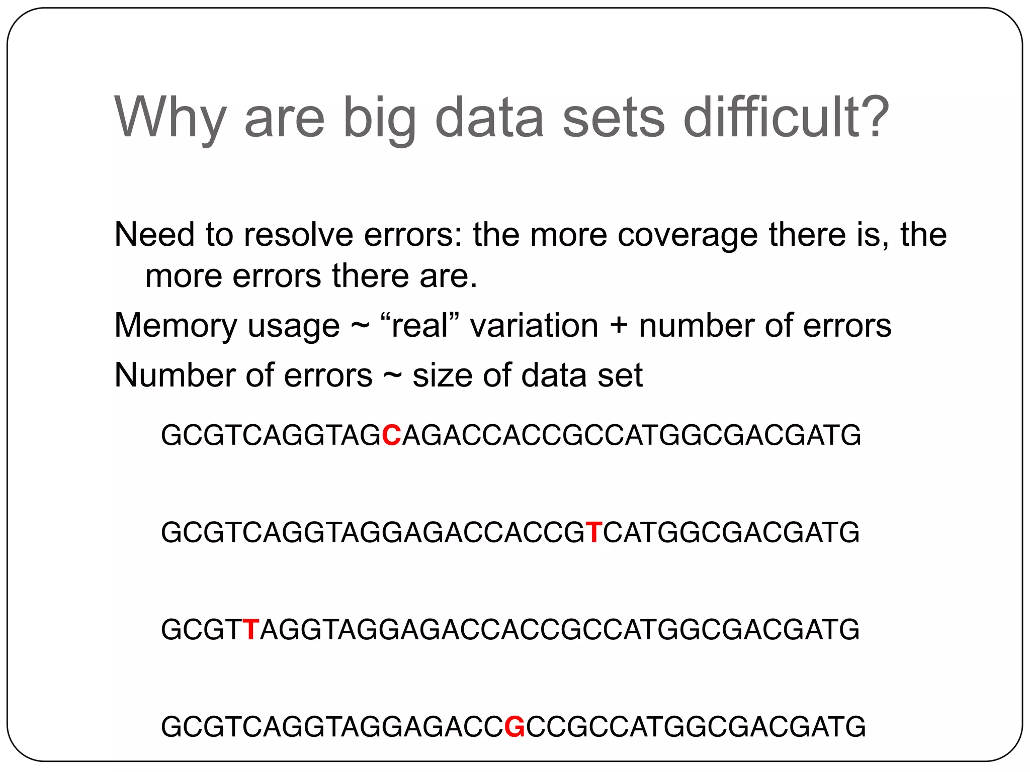
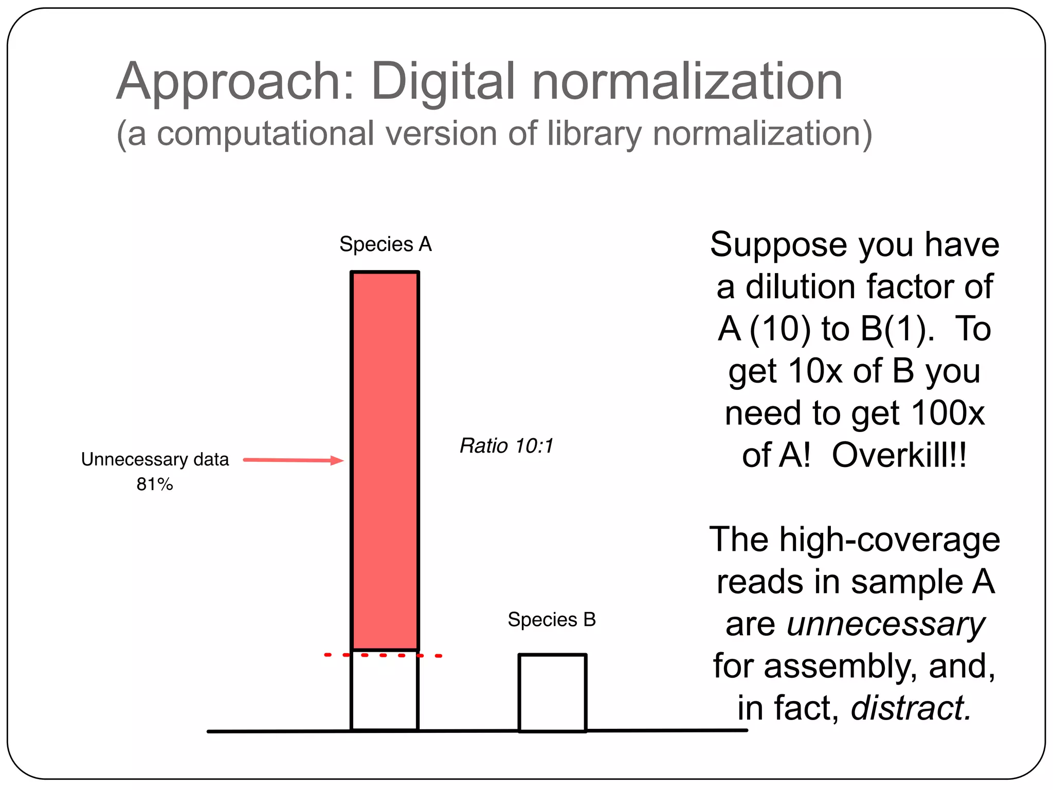
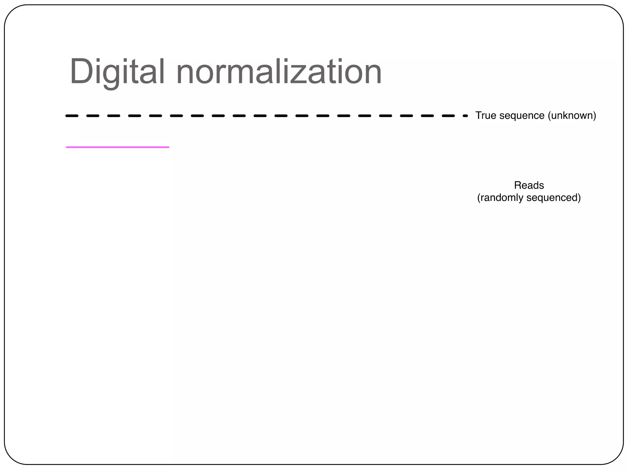
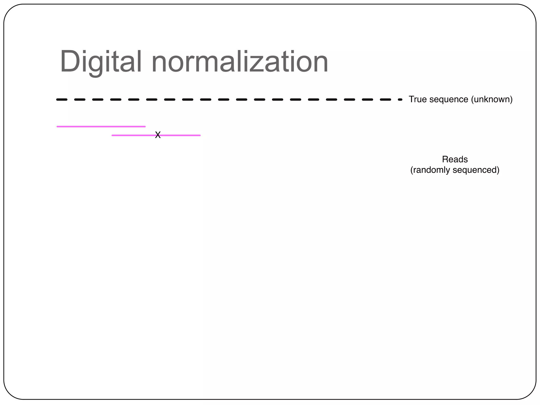
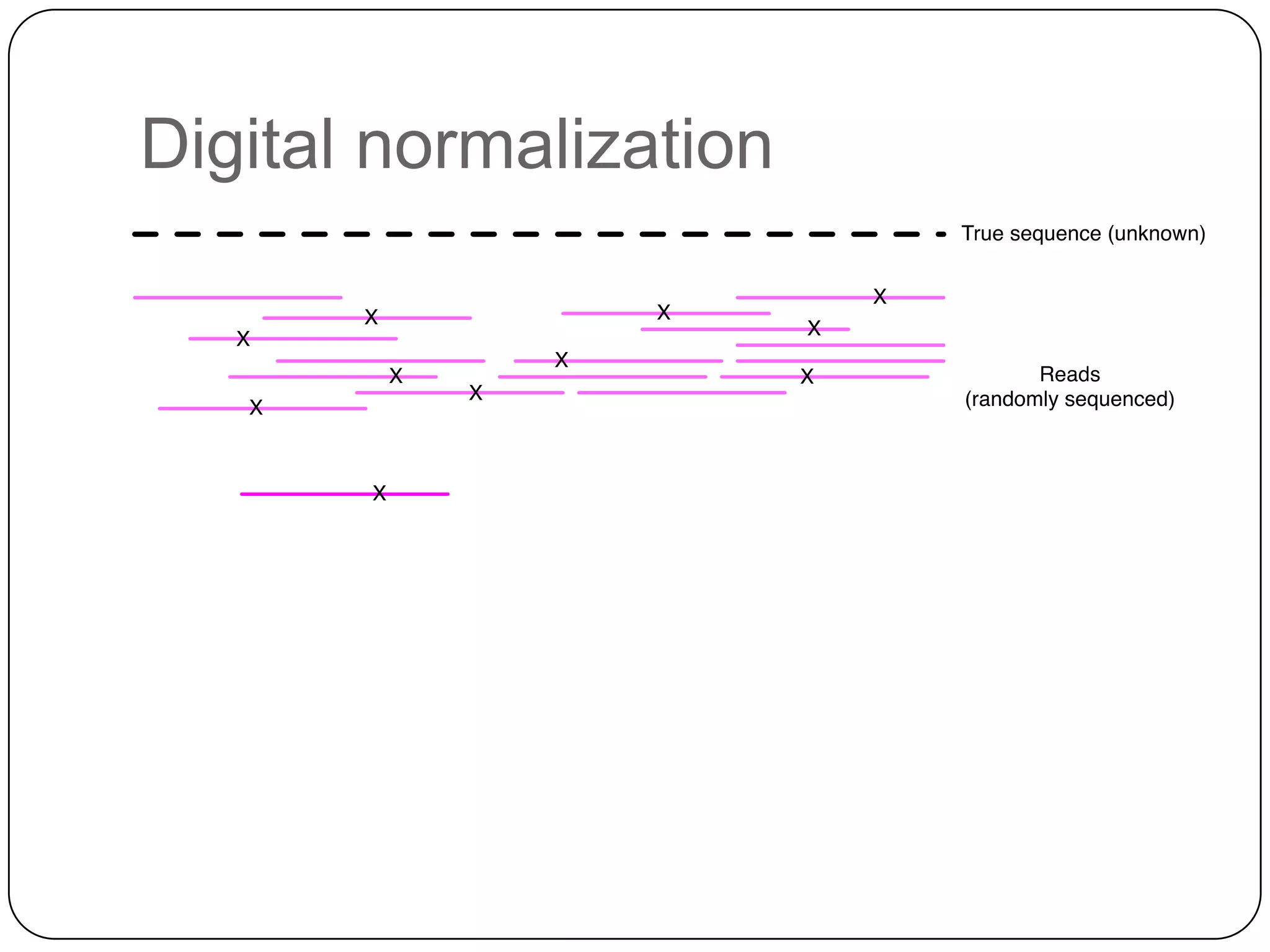
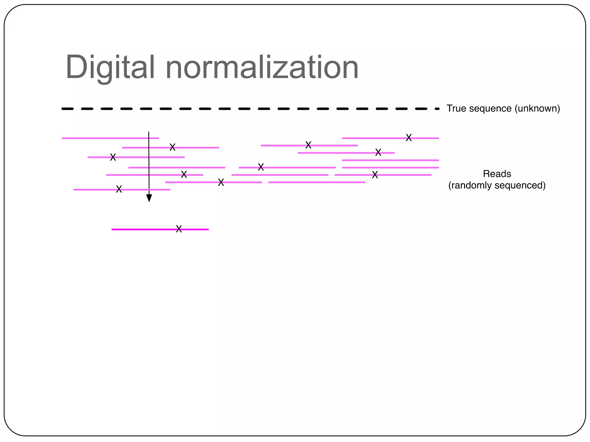
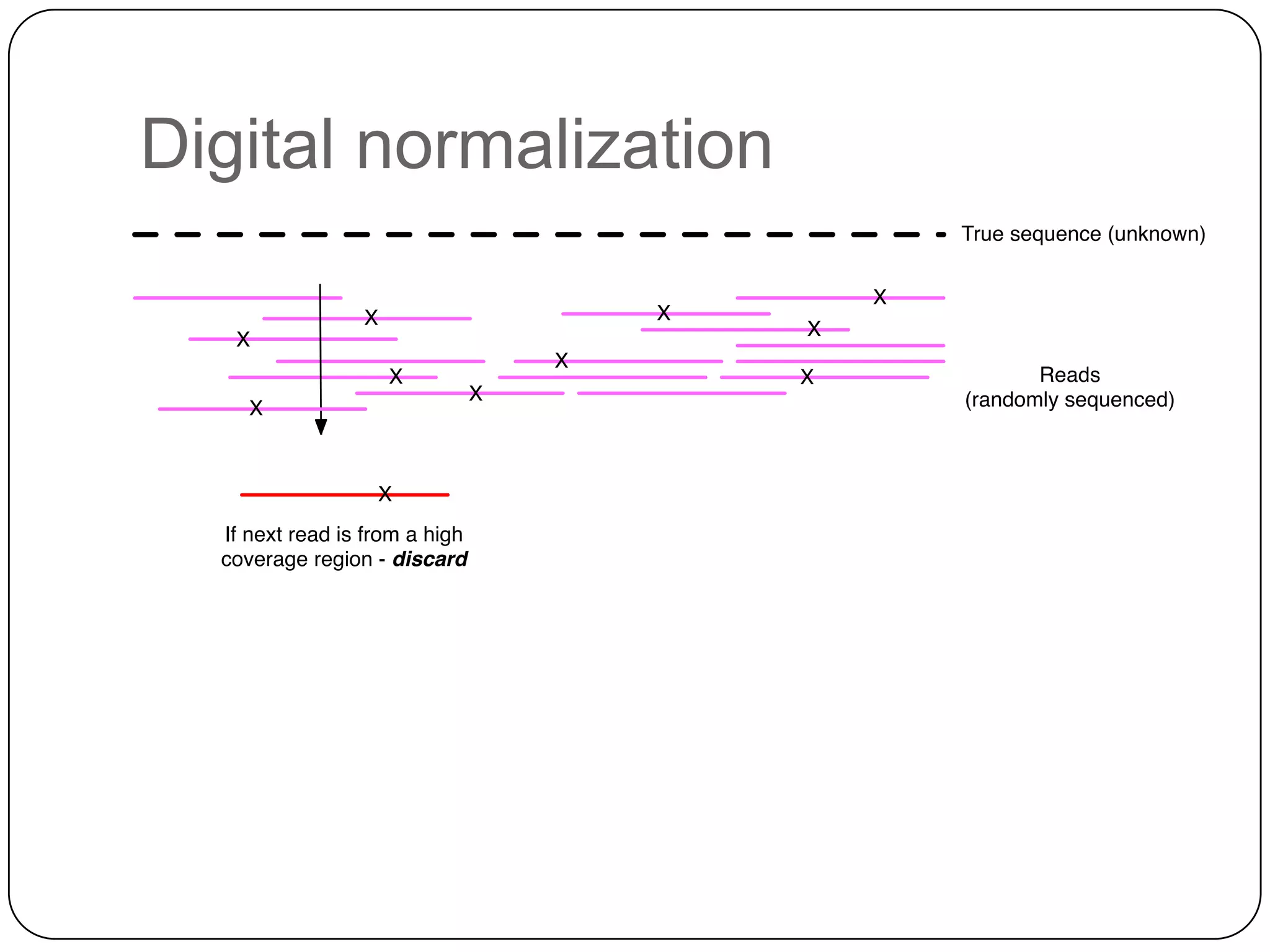
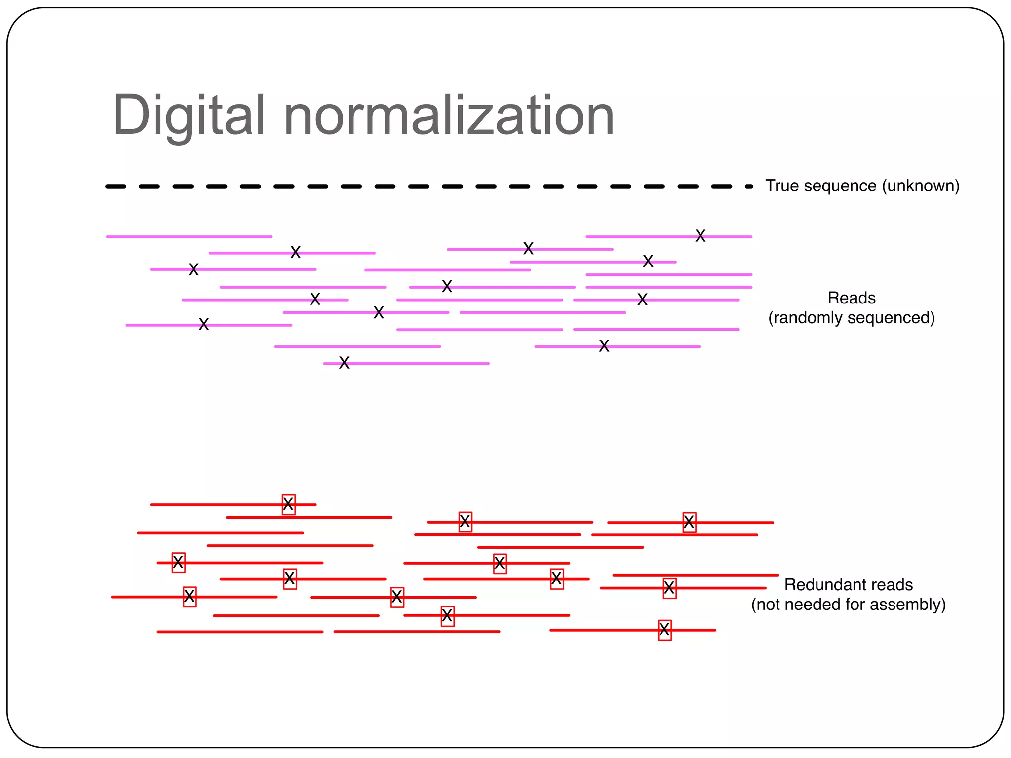
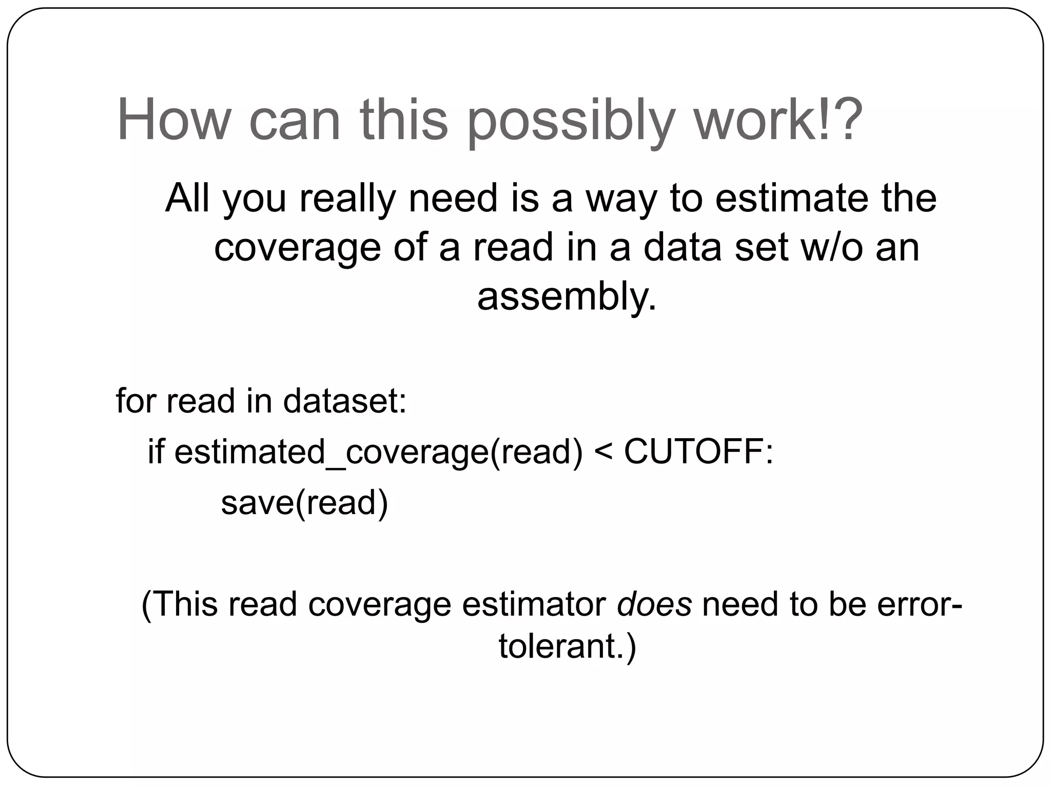
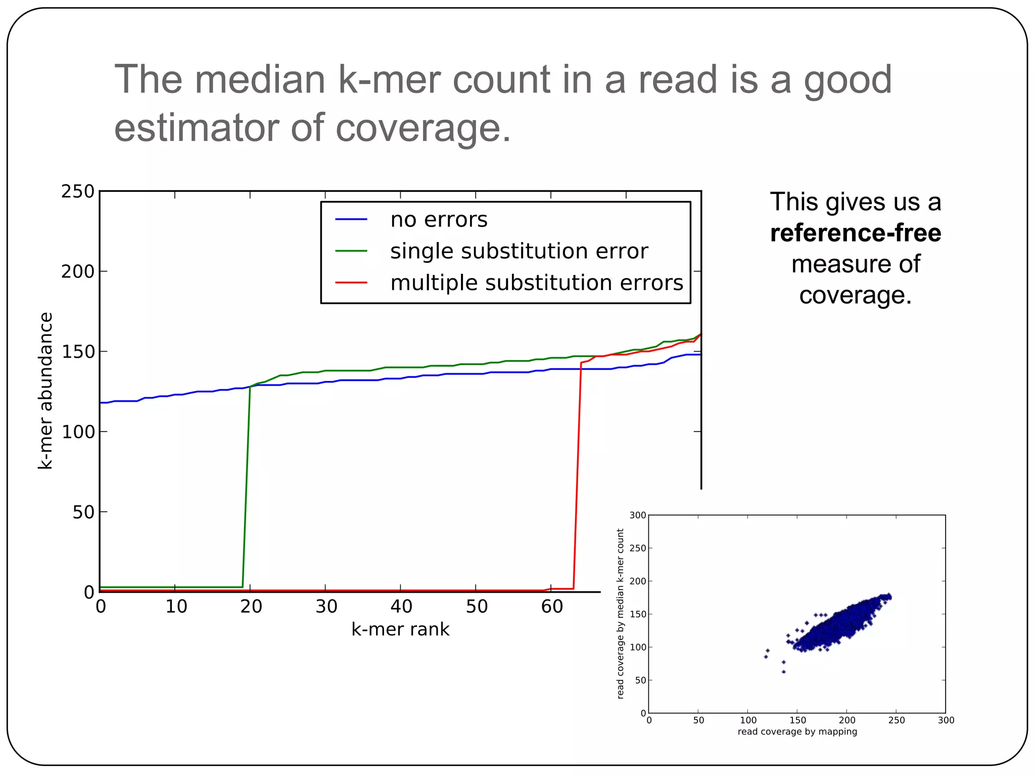
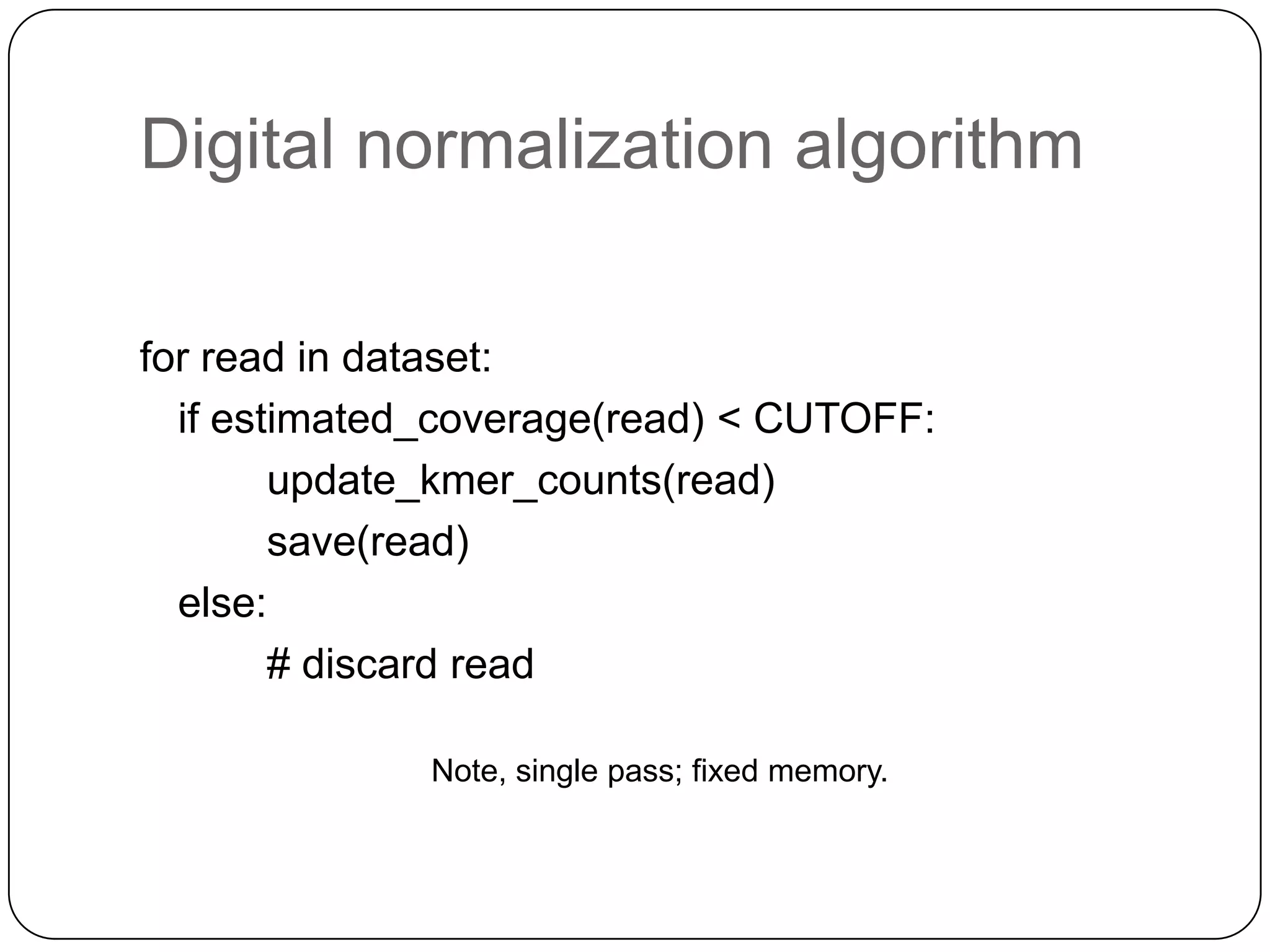
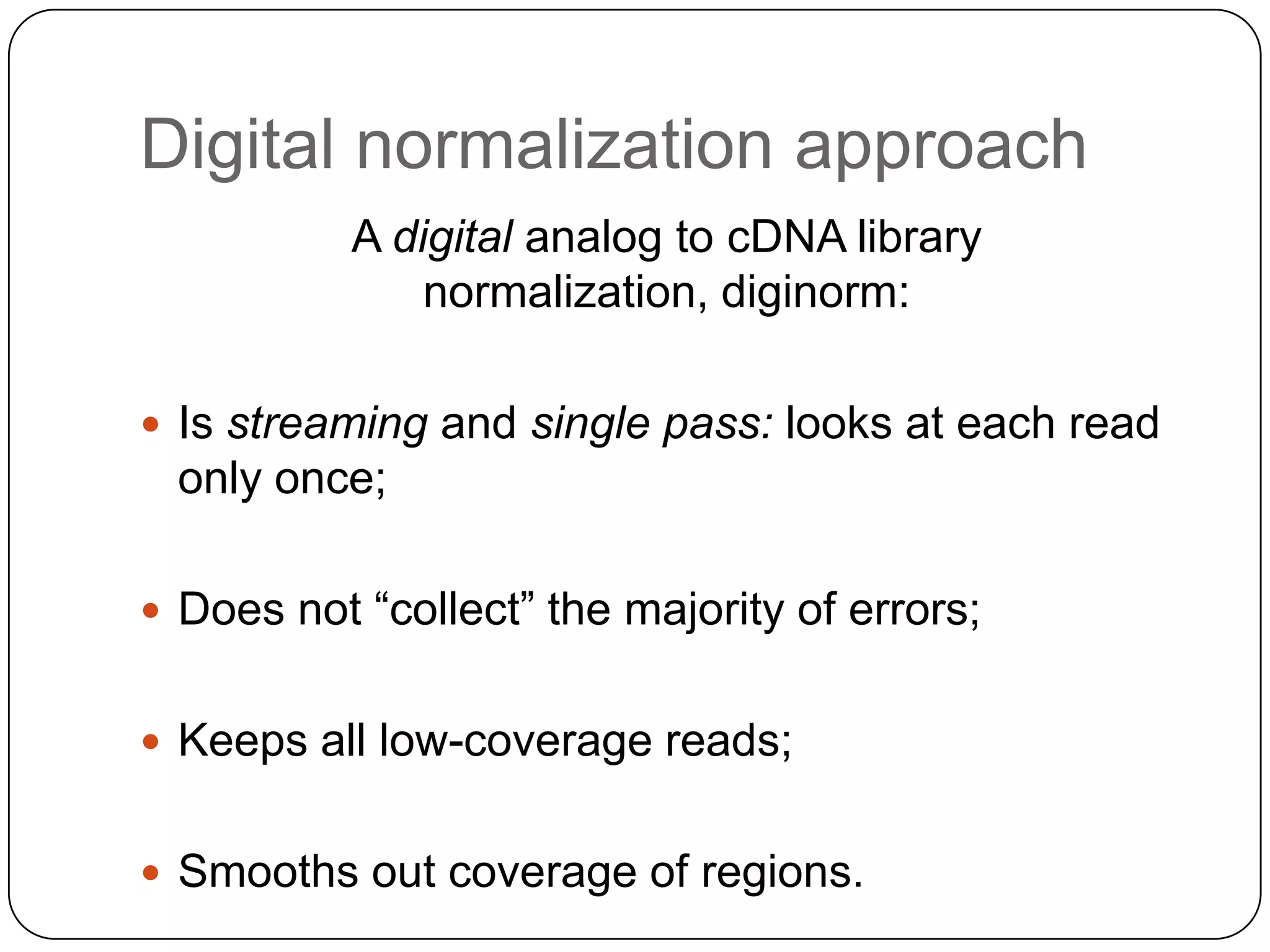
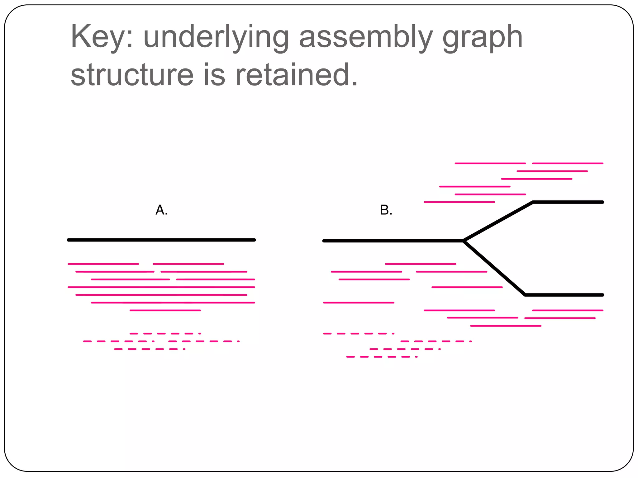
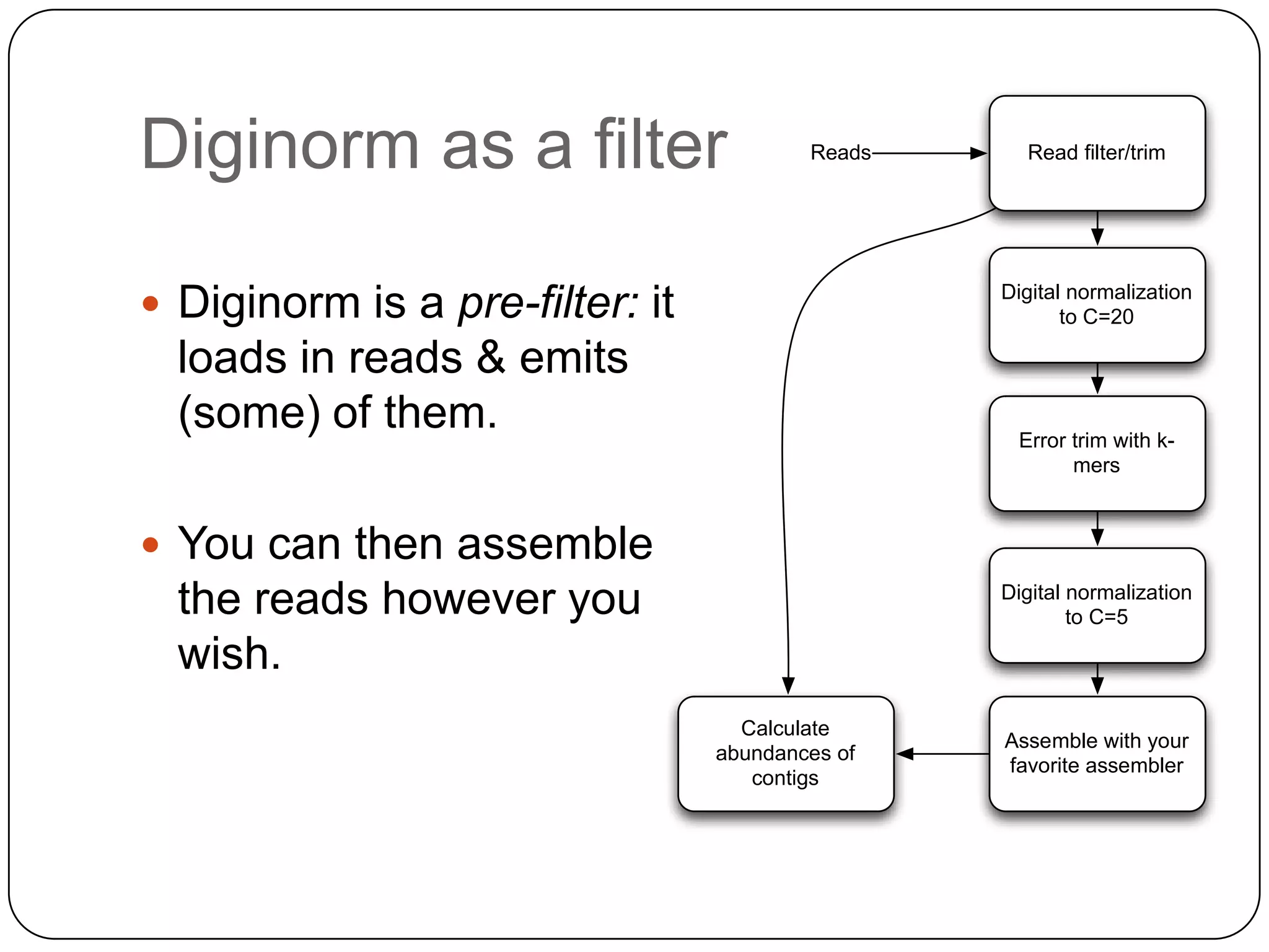
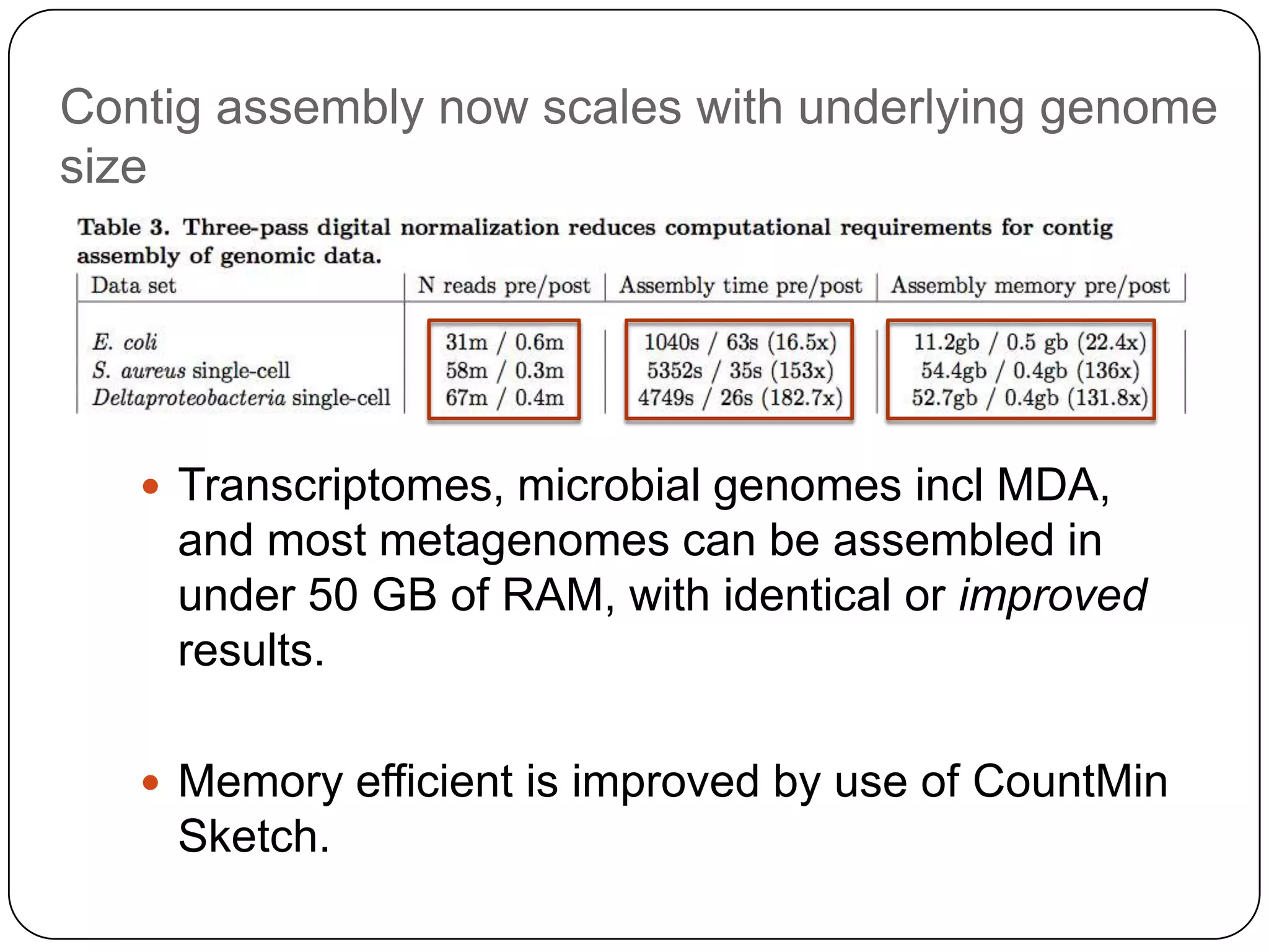
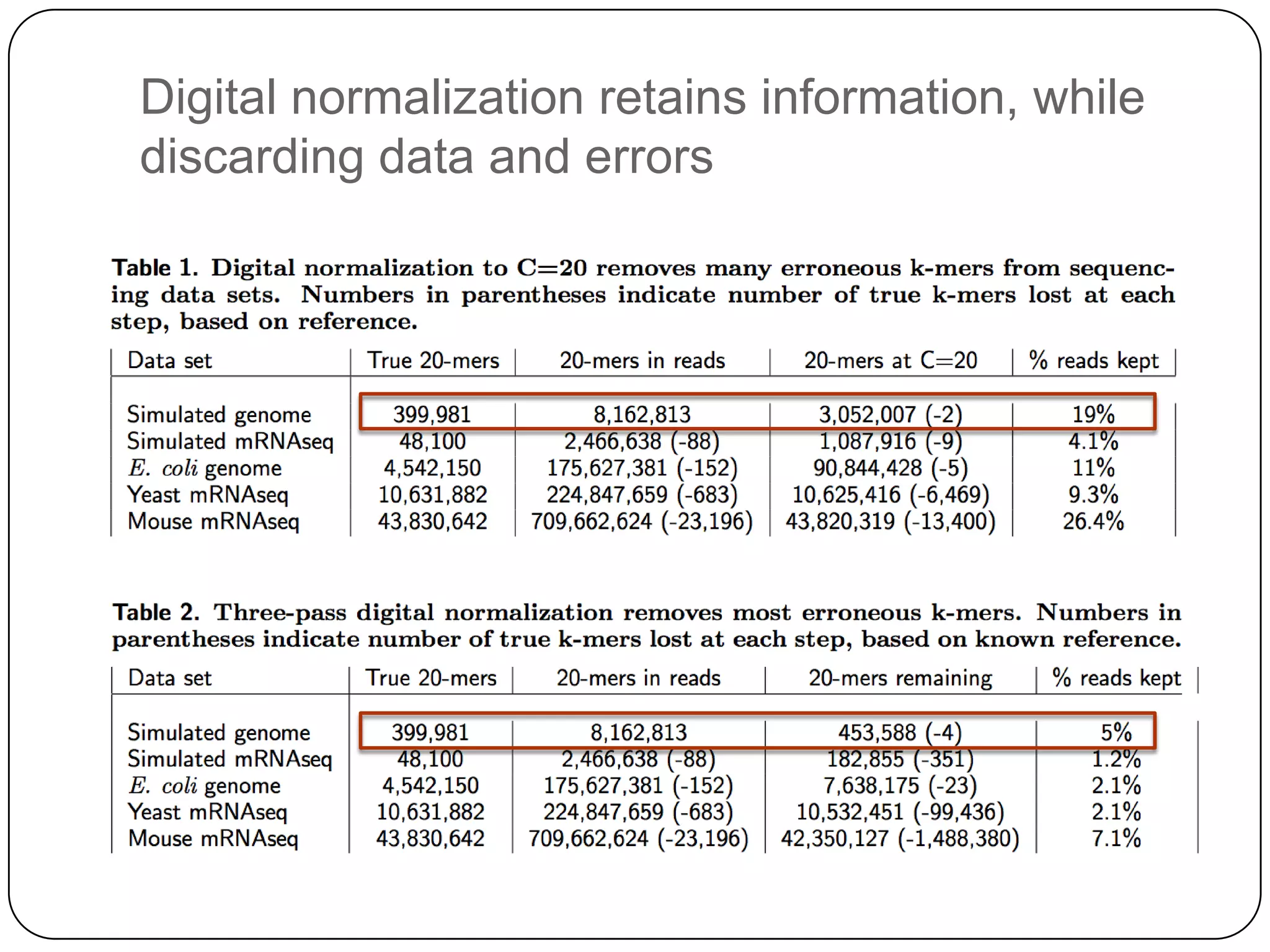
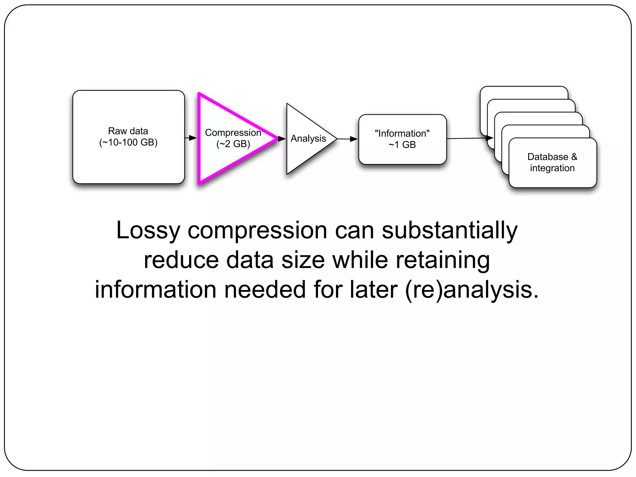
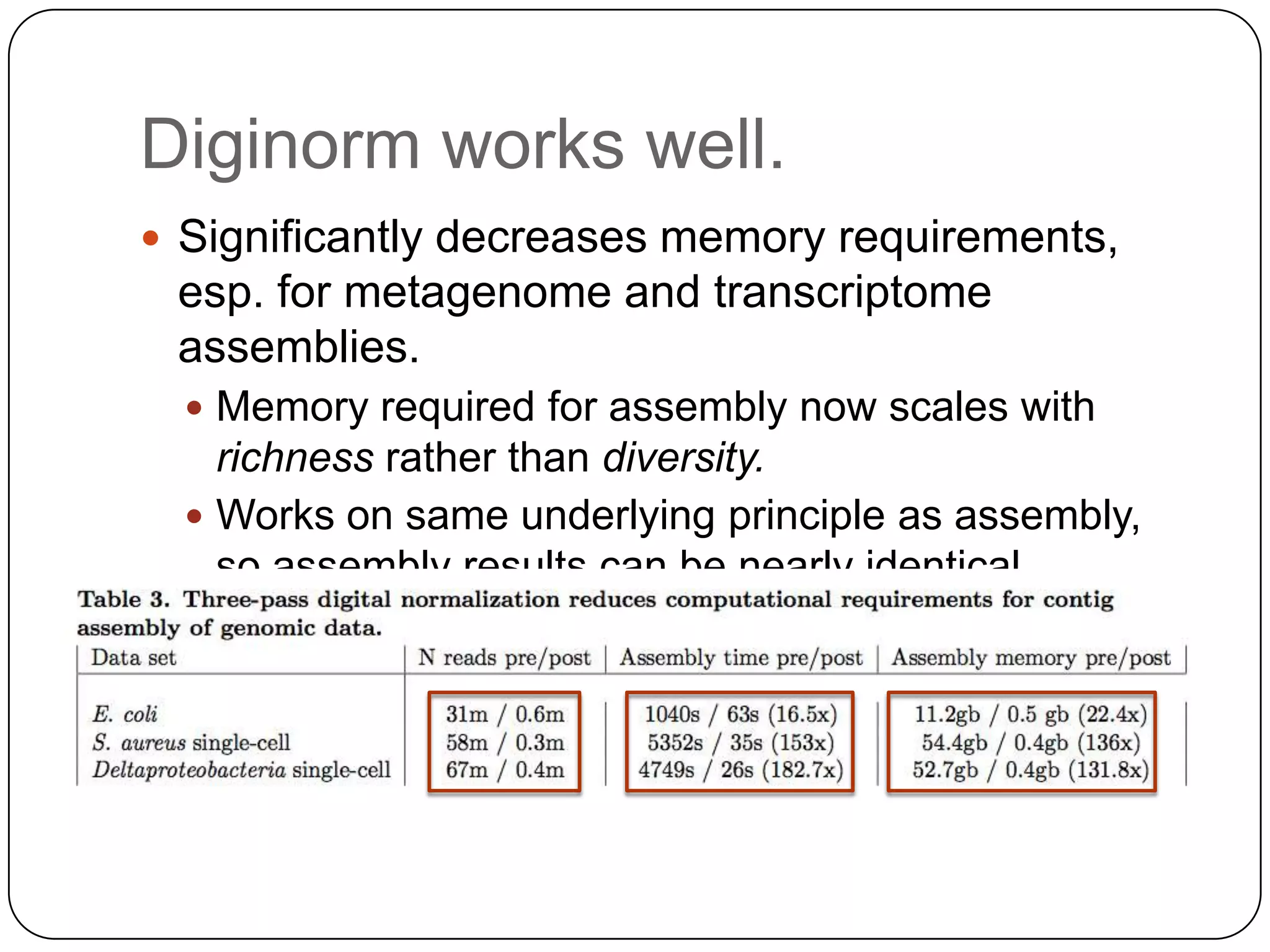
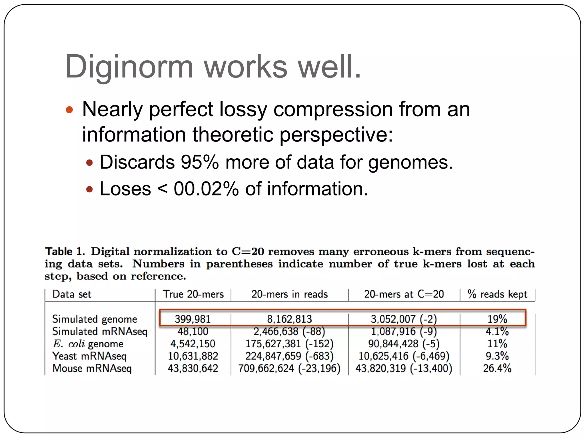
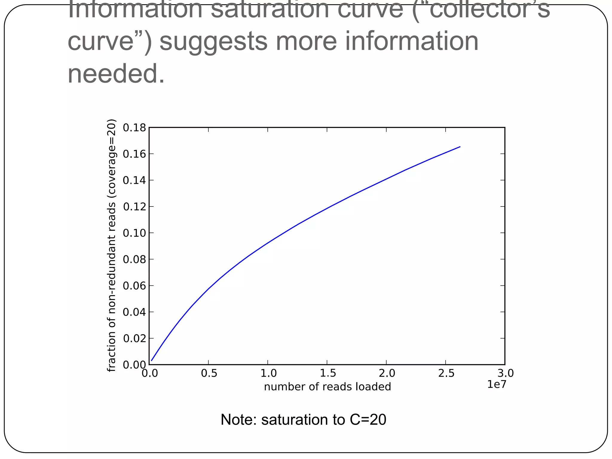
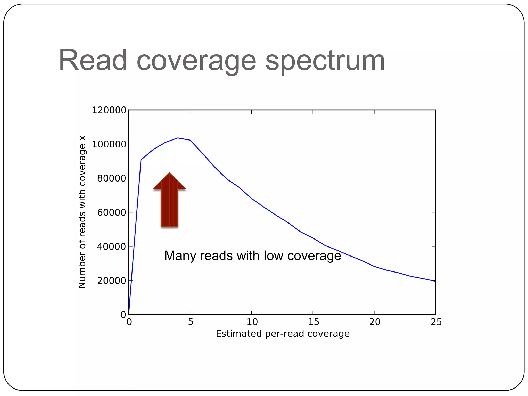
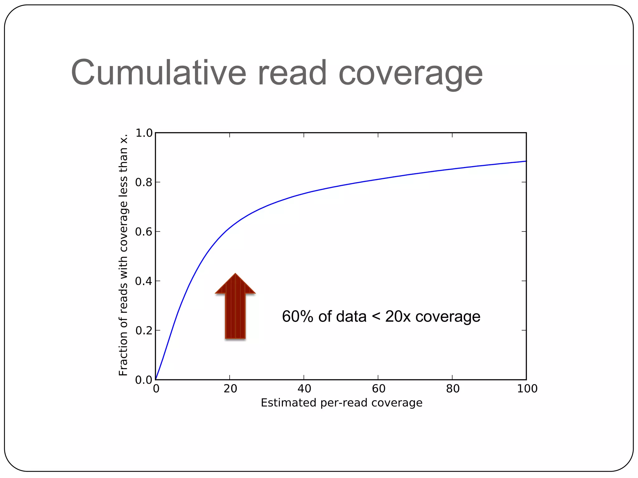
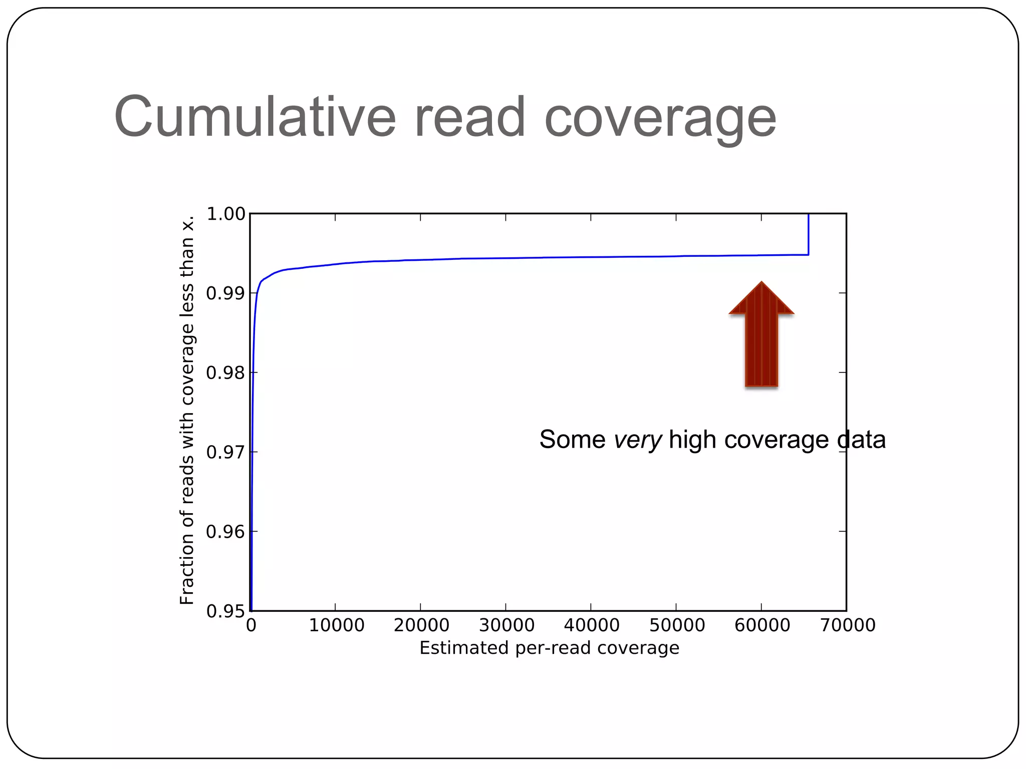
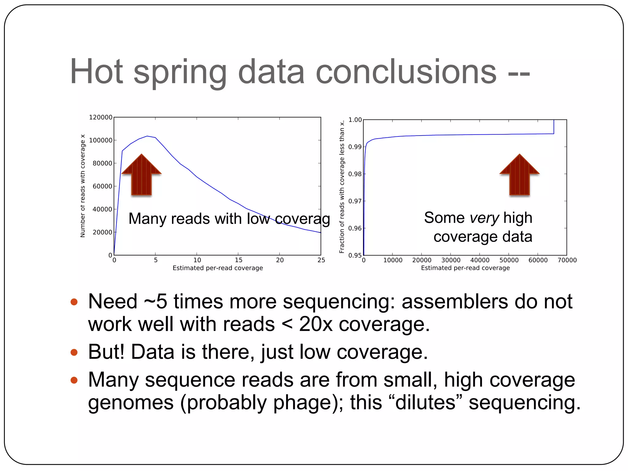
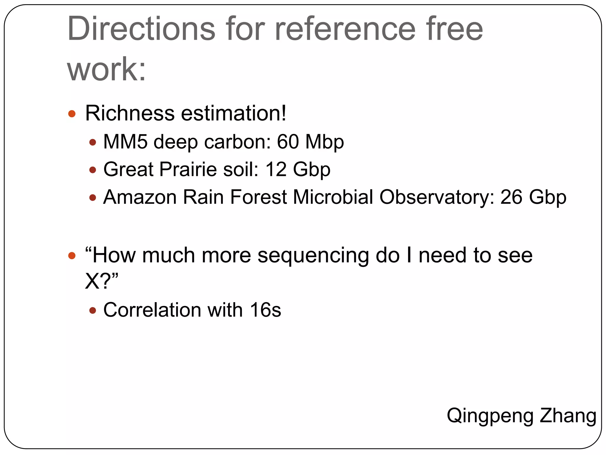
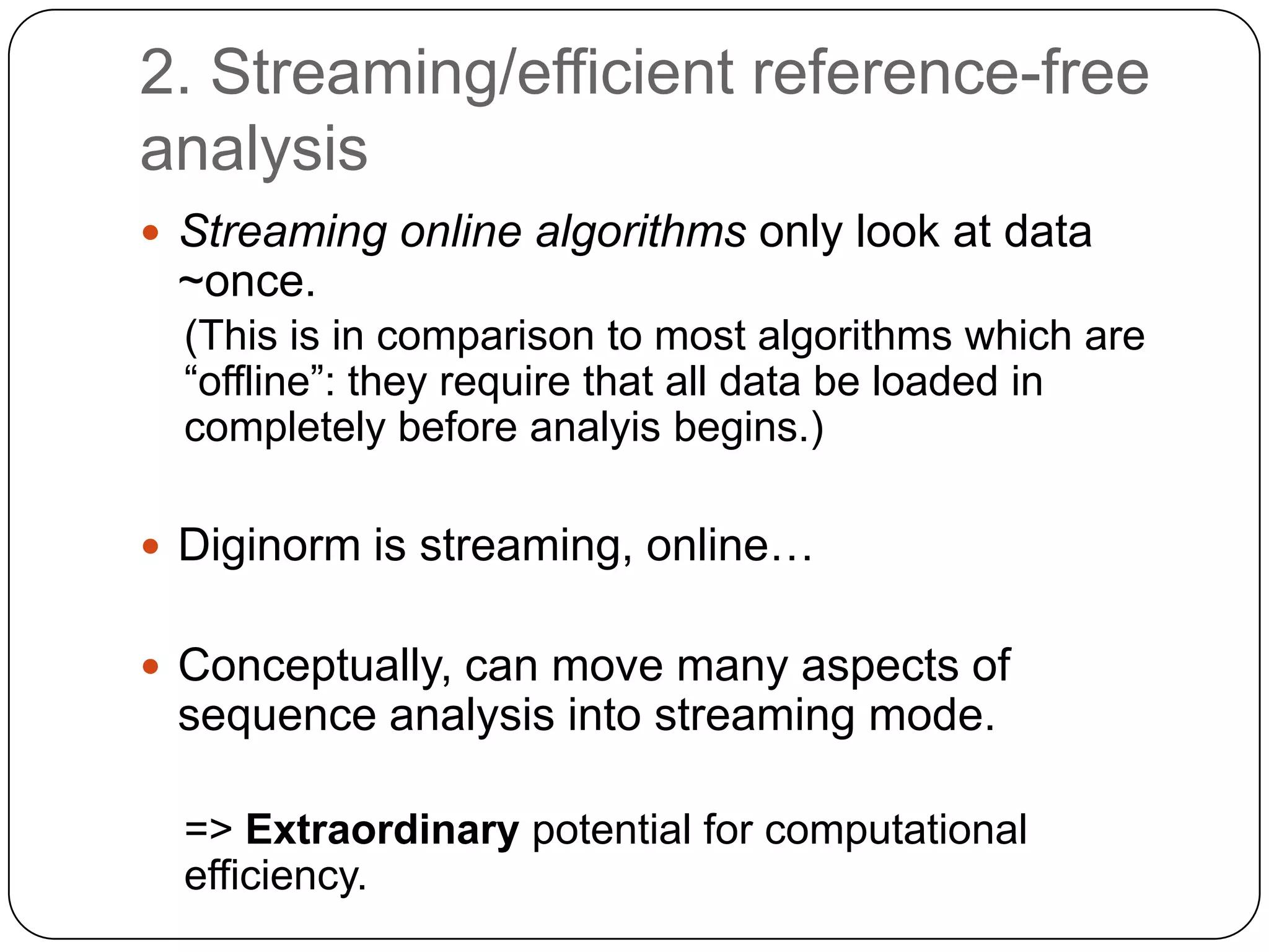
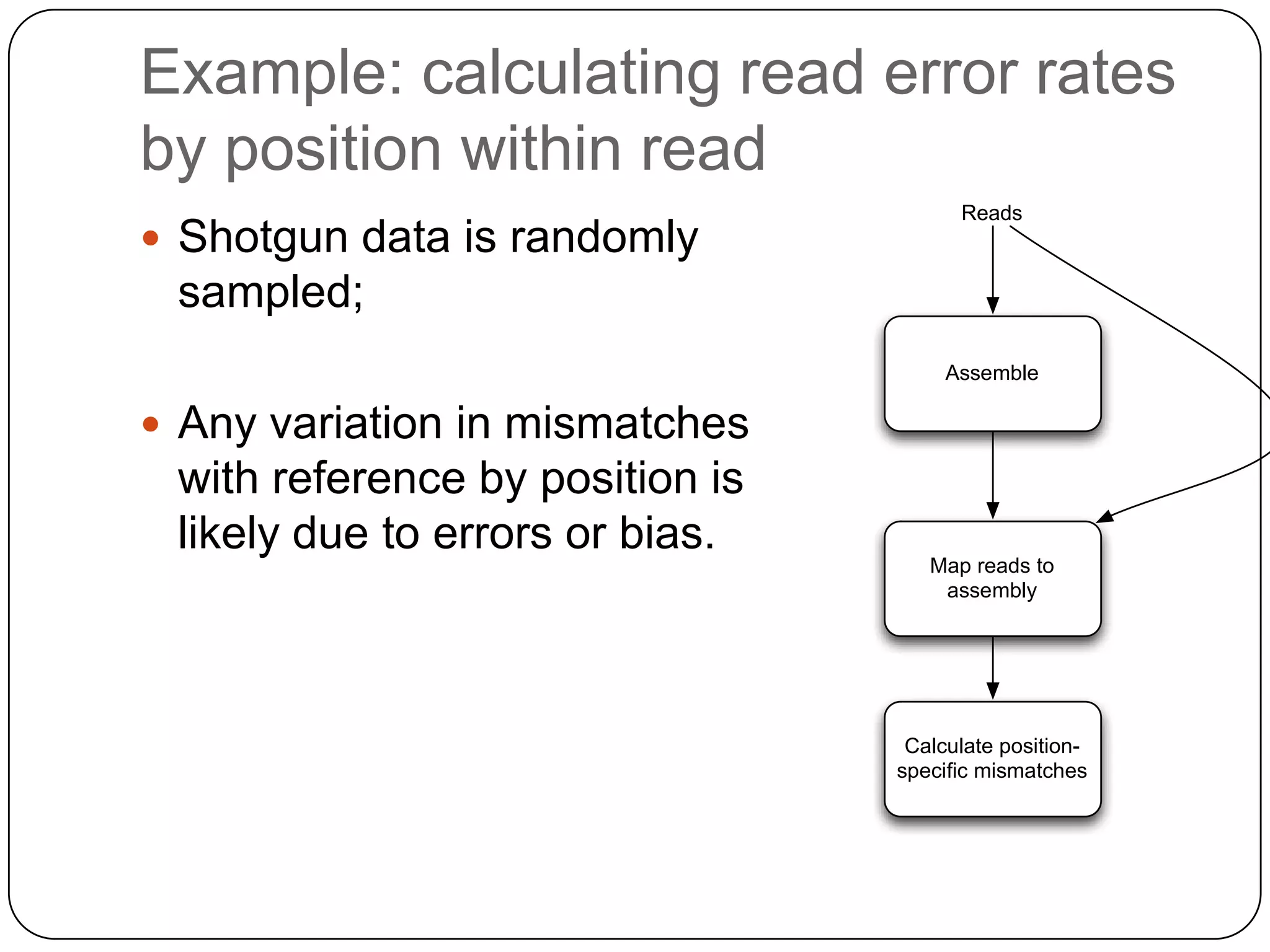
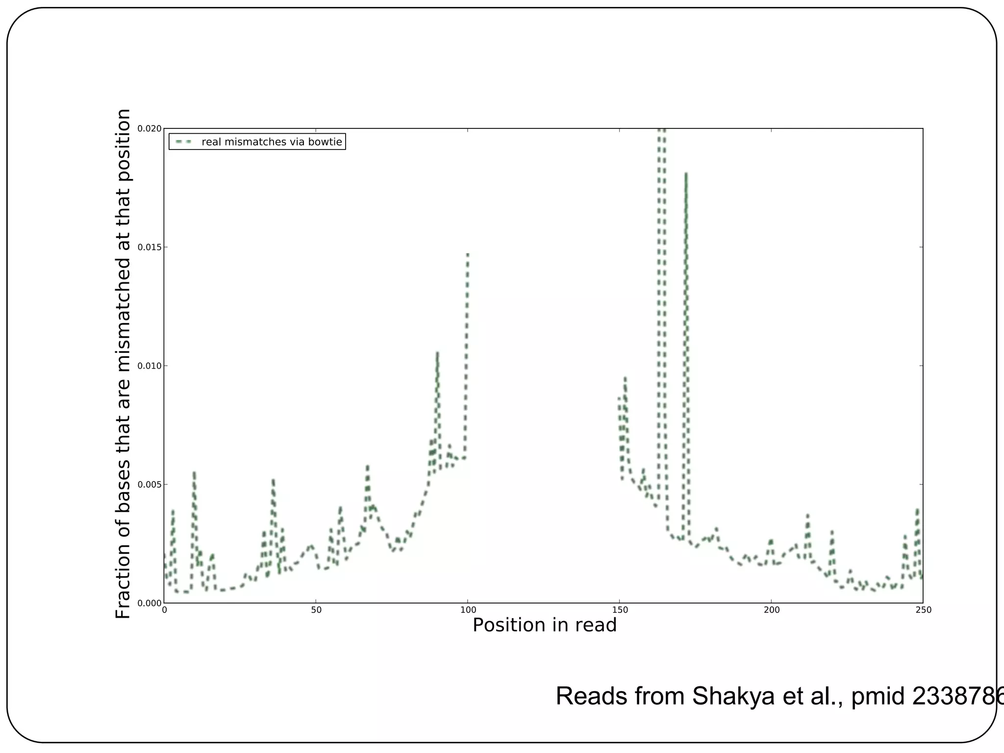
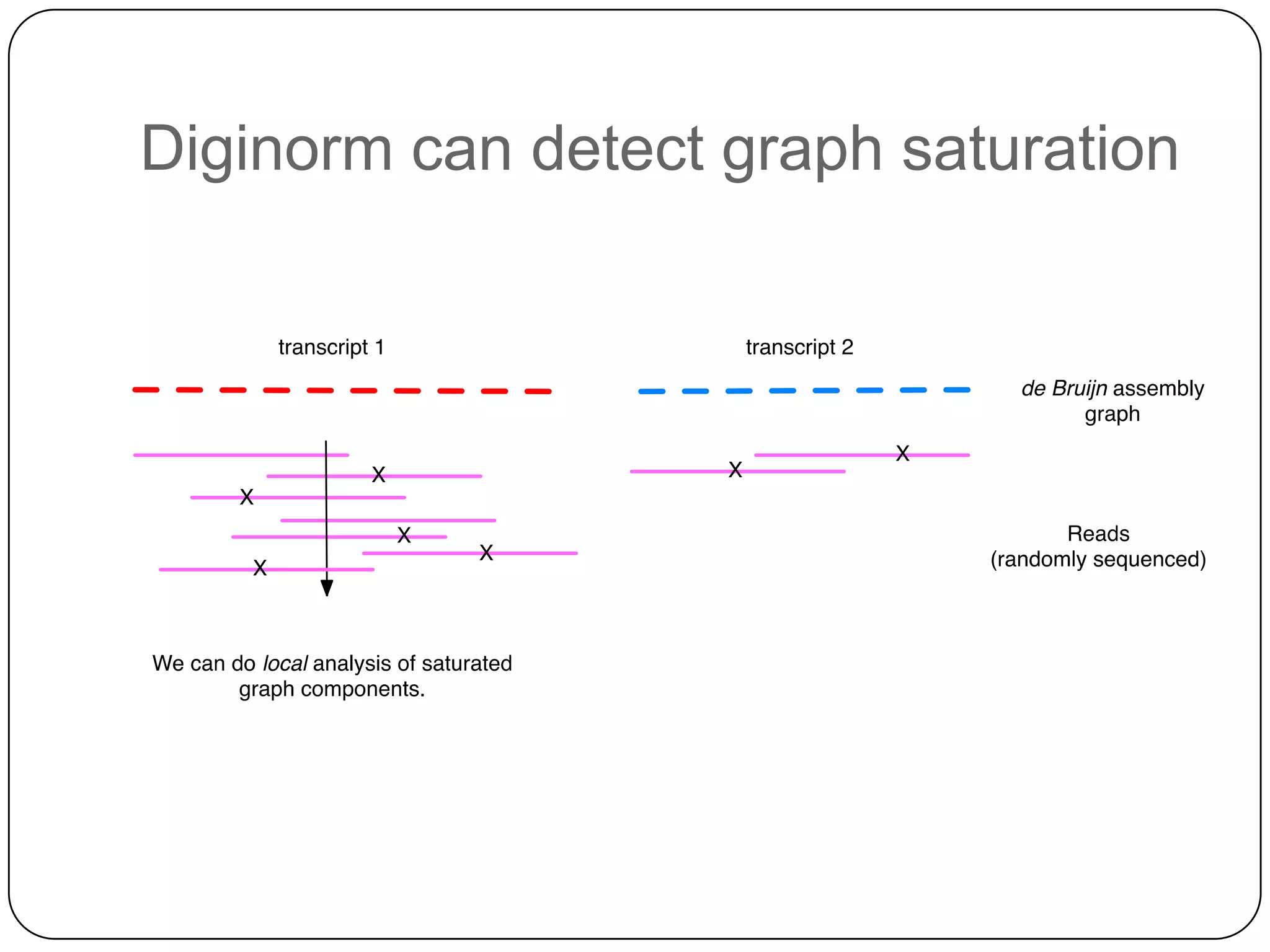
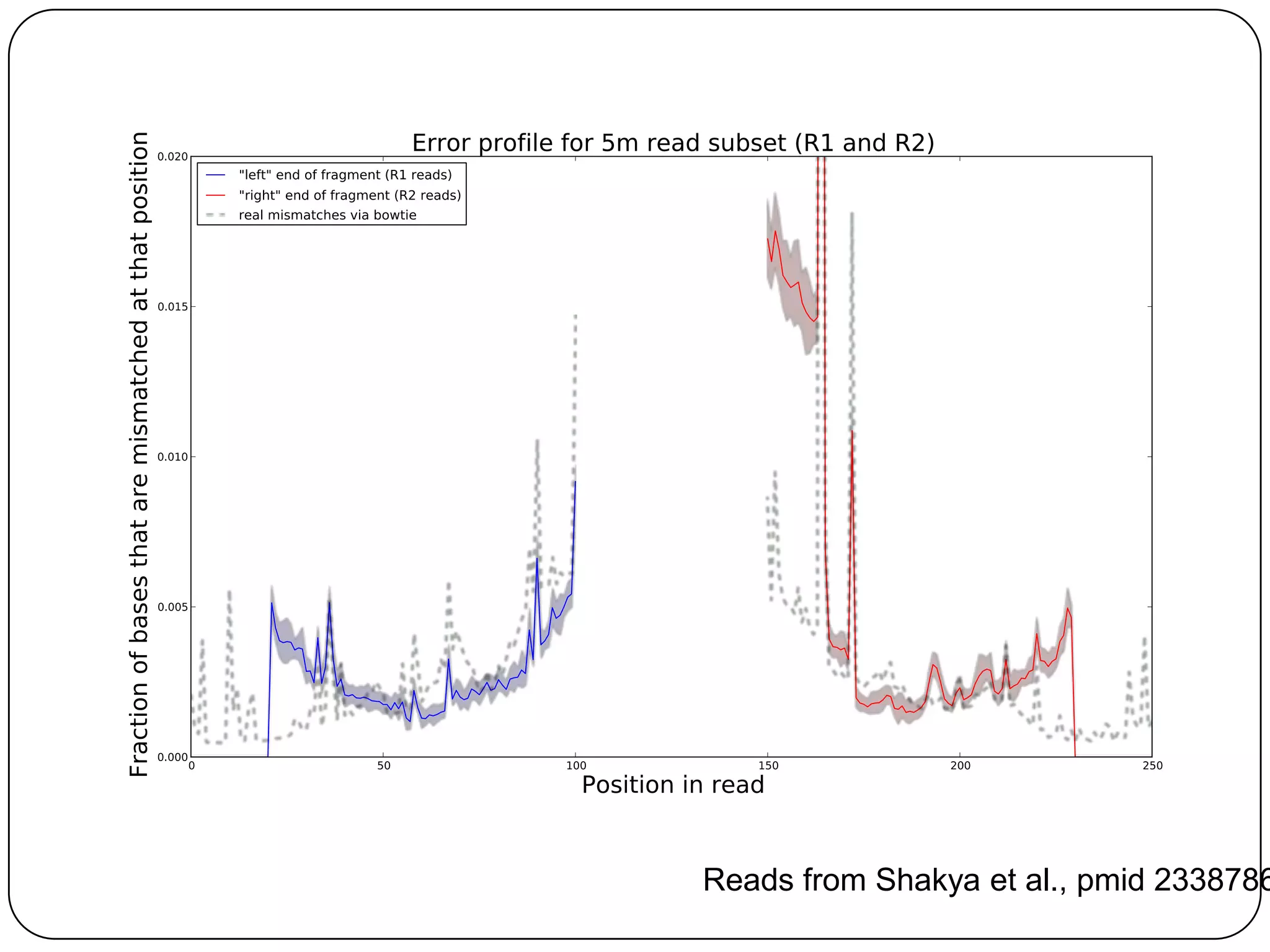
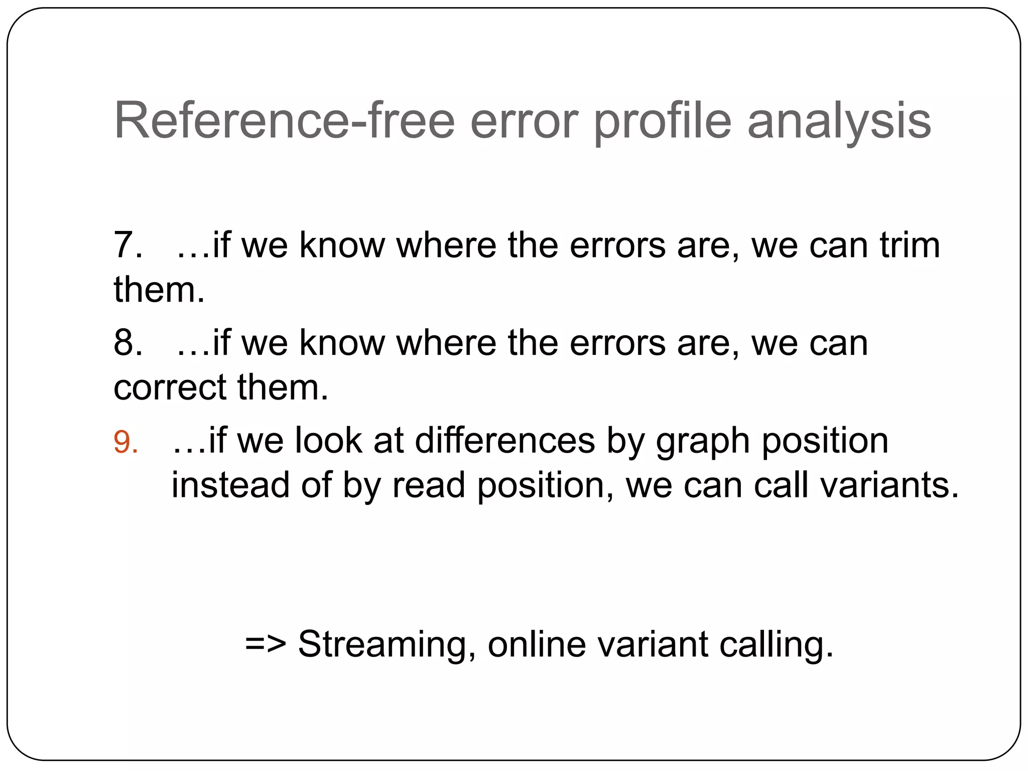
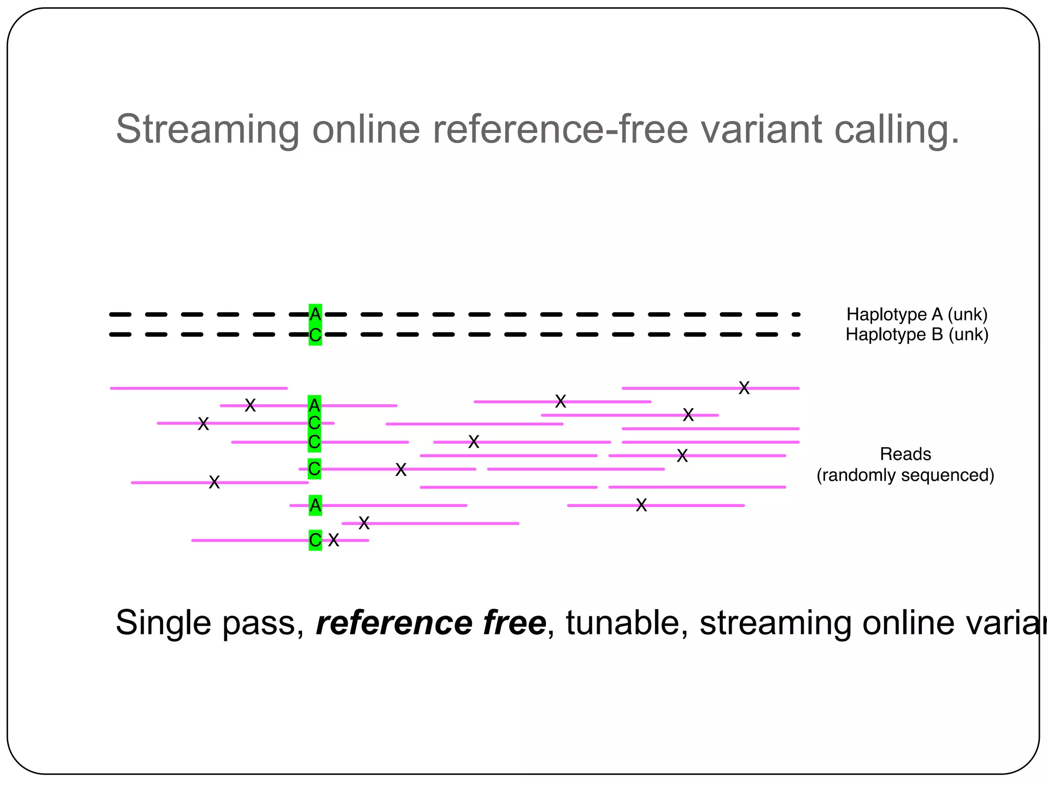
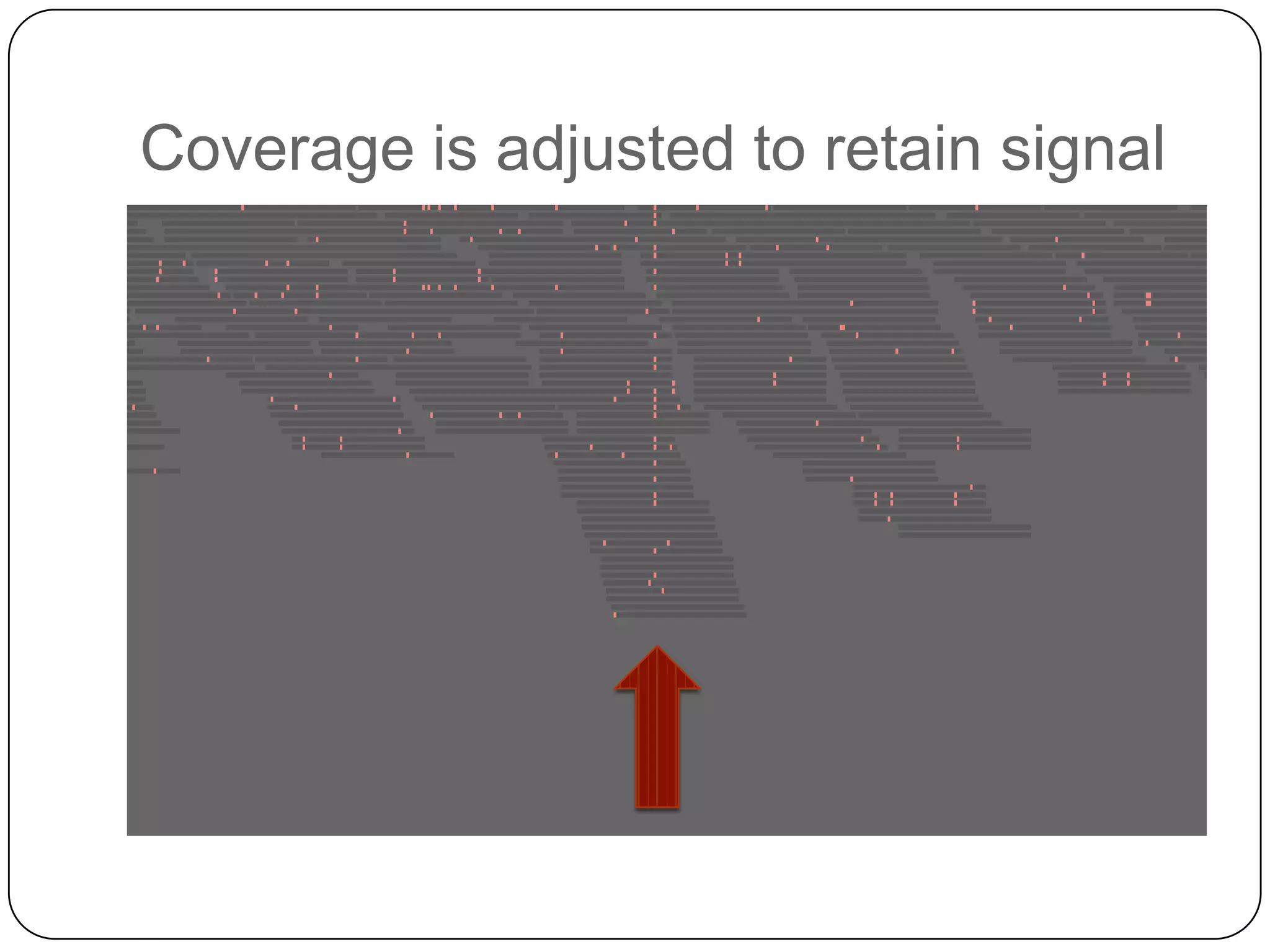
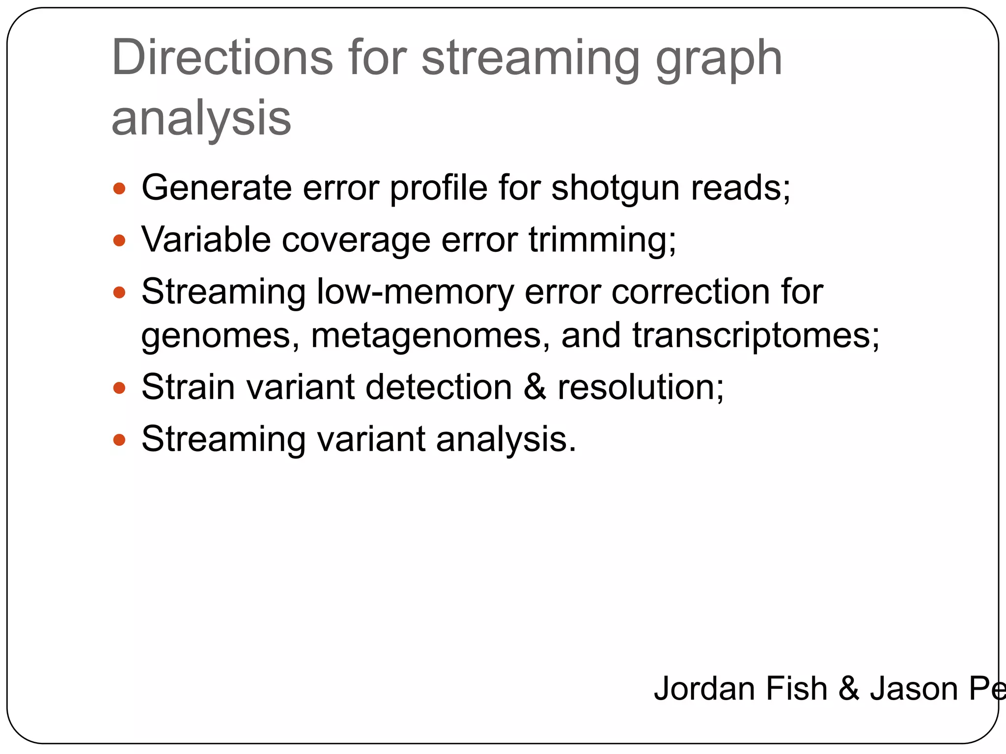
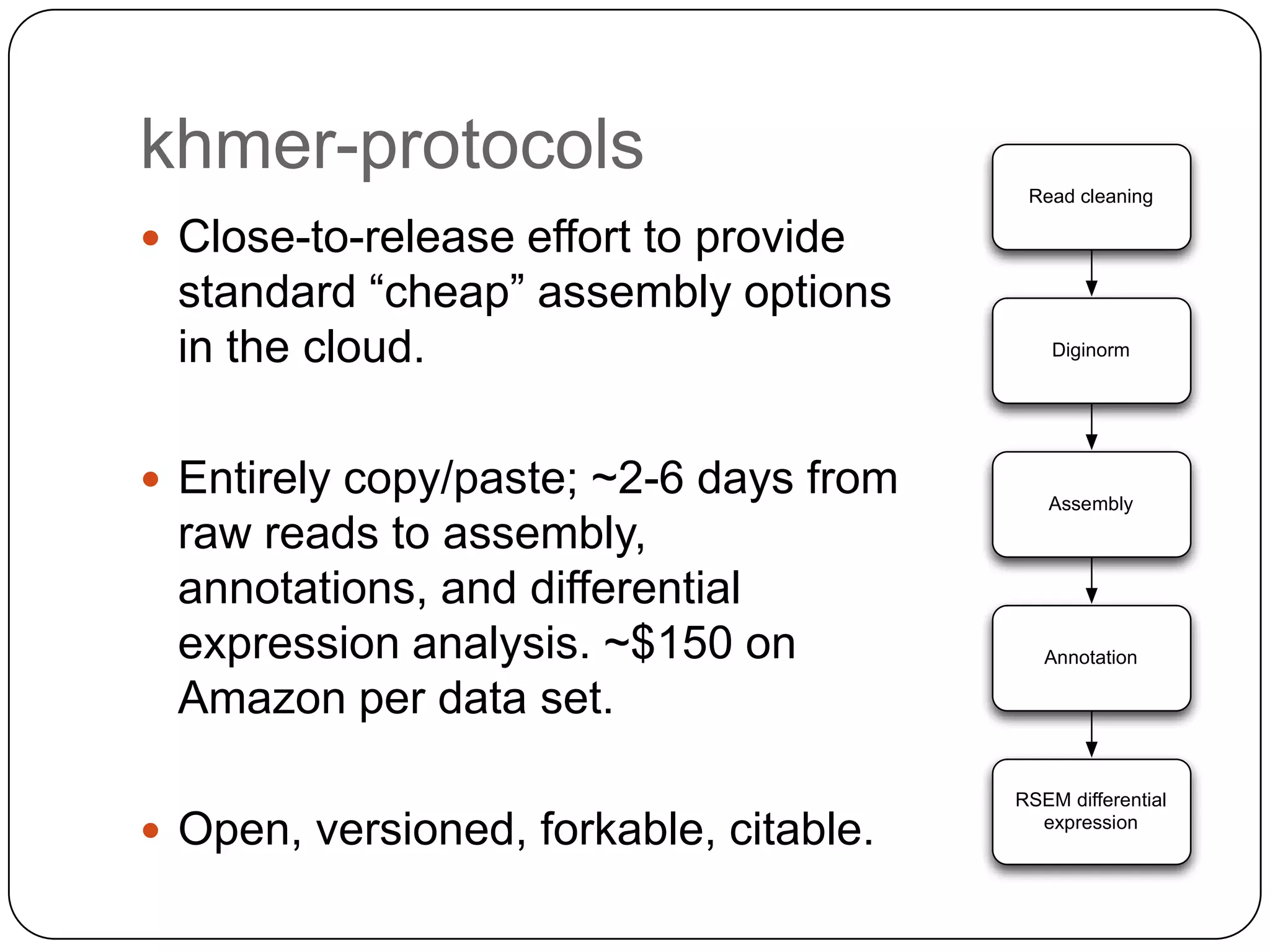
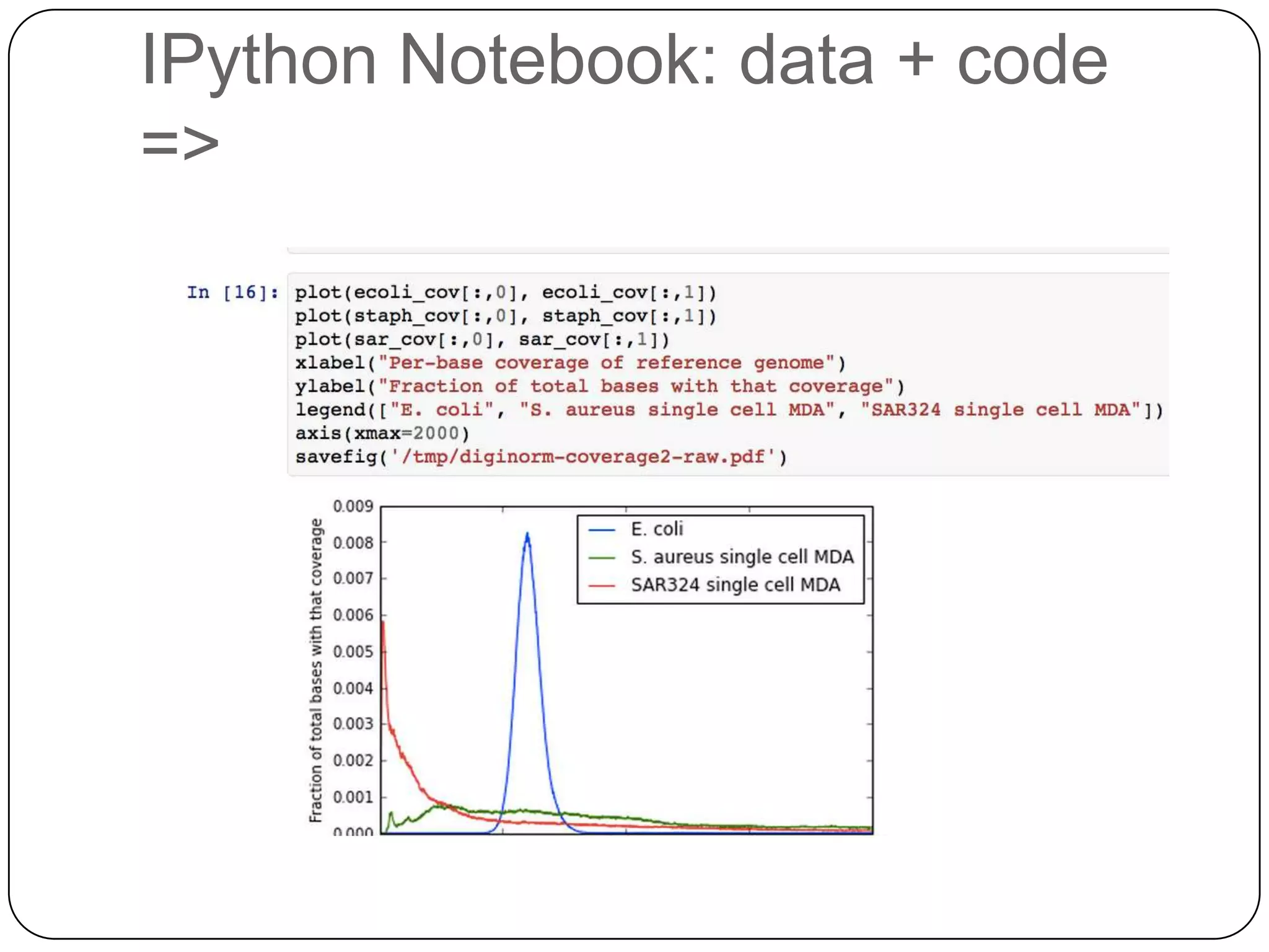
Digital normalization provides a computationally efficient way to filter high-coverage reads from shotgun sequencing data, reducing data size while retaining most of the information needed for downstream analysis. It works by estimating the coverage of each read without using a reference genome and discarding reads above a given coverage cutoff. The method has been shown to significantly decrease memory requirements for de novo assembly of various data types like metagenomes and transcriptomes, while producing similar or improved assembly results. Future work includes developing reference-free methods for analyzing sequencing data in a streaming fashion before or without assembly.

1. Digital normalization and some consequences.
C. Titus Brown
Assistant Professor
CSE, MMG, BEACON
Michigan State University
Nov 2013
ctb@msu.edu

2. Acknowledgements
Lab members involved
Collaborators
 Adina Howe (w/Tiedje)
 Jim Tiedje, MSU
 Erich Schwarz, Caltech /
 Jason Pell
 Arend Hintze
 Rosangela Canino-Koning
 Qingpeng Zhang
 Elijah Lowe
 Likit Preeyanon
 Jiarong Guo
 Tim Brom
 Kanchan Pavangadkar
 Eric McDonald
 Chris Welcher
 Michael Crusoe
Cornell
 Paul Sternberg, Caltech
 Robin Gasser, U.
Melbourne
 Weiming Li
Funding
USDA NIFA; NSF IOS;
NIH; BEACON.

3. We practice open science!
“Be the change you want”
Everything discussed here:
 Code: github.com/ged-lab/ ; BSD license
 Blog: http://ivory.idyll.org/blog („titus brown blog‟)
 Twitter: @ctitusbrown
 Grants on Lab Web site:
http://ged.msu.edu/interests.html
 Preprints: on arXiv, q-bio:
„diginorm arxiv‟

5. Outline
Digital normalization basics
2. Diginorm as streaming lossy compression of
NGS data…
3. …surprisingly useful.
1.
Three new directions:
4.
Reference-free data set investigation
2. Streaming algorithms
3. Open protocols
1.

6. Philosophy: hypothesis generation is
important.
 We need better methods to investigate and
analyze large sequencing data sets.
 To be most useful, these methods should be fast
& computationally efficient, because:
 Data gathering rate is already quite high
 Allows iterations
 Better methods for good computational
hypothesis generation are critical to moving
forward.

7. High-throughput sequencing
 I mostly work on ecologically and evolutionarily
interesting organisms.
 This includes non-model transcriptomes and
environmental metagenomes.
 Volume of data is a huge problem because of the
diversity of these samples, and because
assembly must be applied to them.

8. Why are big data sets difficult?
Need to resolve errors: the more coverage there is, the
more errors there are.
Memory usage ~ “real” variation + number of errors
Number of errors ~ size of data set

9. There is quite a bit of life left to sequence & assem
http://pacelab.colorado.edu/

10. Shotgun sequencing and
coverage
“Coverage” is simply the average number of reads that overlap
each true base in genome.
Here, the coverage is ~10 – just draw a line straight down from the
top through all of the reads.

11. Random sampling => deep sampling
needed
Typically 10-100x needed for robust recovery (300 Gbp for human)

12. Mixed populations.
 Approximately 20-40x coverage is required to
assemble the majority of a bacterial genome from
short reads. 100x is required for a “good” assembly.
 To sample a mixed population thoroughly, you need to
sample 100x of the lowest abundance species
present.
 For example, for E. coli in 1/1000 dilution, you would
need approximately 100x coverage of a 5mb genome
at 1/1000, or 500 Gbp of sequence!
 …actually getting this much sequence is fairly easy,
but is then hard to assemble in a reasonable
computer.

13. Approach: Digital normalization
(a computational version of library normalization)
Suppose you have
a dilution factor of
A (10) to B(1). To
get 10x of B you
need to get 100x
of A! Overkill!!
The high-coverage
reads in sample A
are unnecessary
for assembly, and,
in fact, distract.

14. Digital normalization

15. Digital normalization

16. Digital normalization

17. Digital normalization

18. Digital normalization

19. Digital normalization

20. How can this possibly work!?
All you really need is a way to estimate the
coverage of a read in a data set w/o an
assembly.
for read in dataset:
if estimated_coverage(read) < CUTOFF:
save(read)
(This read coverage estimator does need to be errortolerant.)

21. The median k-mer count in a read is a good
estimator of coverage.
This gives us a
reference-free
measure of
coverage.

22. Digital normalization algorithm
for read in dataset:
if estimated_coverage(read) < CUTOFF:
update_kmer_counts(read)
save(read)
else:
# discard read
Note, single pass; fixed memory.

23. Digital normalization approach
A digital analog to cDNA library
normalization, diginorm:
 Is streaming and single pass: looks at each read
only once;
 Does not “collect” the majority of errors;
 Keeps all low-coverage reads;
 Smooths out coverage of regions.

24. Key: underlying assembly graph
structure is retained.

25. Diginorm as a filter
Reads
Read filter/trim
Digital normalization
to C=20
 Diginorm is a pre-filter: it
loads in reads & emits
(some) of them.
Error trim with kmers
 You can then assemble
the reads however you
wish.
Digital normalization
to C=5
Calculate
abundances of
contigs
Assemble with your
favorite assembler

26. Contig assembly now scales with underlying genome
size
 Transcriptomes, microbial genomes incl MDA,
and most metagenomes can be assembled in
under 50 GB of RAM, with identical or improved
results.
 Memory efficient is improved by use of CountMin
Sketch.

27. Digital normalization retains information, while
discarding data and errors

28. Lossy compression
http://en.wikipedia.org/wiki/JPEG

29. Lossy compression
http://en.wikipedia.org/wiki/JPEG

30. Lossy compression
http://en.wikipedia.org/wiki/JPEG

31. Lossy compression
http://en.wikipedia.org/wiki/JPEG

32. Lossy compression
http://en.wikipedia.org/wiki/JPEG

33. Raw data
(~10-100 GB)
Compression
(~2 GB)
Analysis
"Information"
~1 GB
"Information"
"Information"
"Information"
"Information"
Database &
integration
Lossy compression can substantially
reduce data size while retaining
information needed for later (re)analysis.

34. Some diginorm examples:
1. Assembly of the H. contortus parasitic nematode
genome, a “high polymorphism/variable coverage”
problem.
(Schwarz et al., 2013; pmid 23985341)
2. Reference-free assembly of the lamprey (P.
marinus) transcriptome, a “big assembly” problem.
(in prep)
3. Assembly of two Midwest soil metagenomes,
Iowa corn and Iowa prairie – the “impossible”
assembly problem.

35. Diginorm works well.
 Significantly decreases memory requirements,
esp. for metagenome and transcriptome
assemblies.
 Memory required for assembly now scales with
richness rather than diversity.
 Works on same underlying principle as assembly,
so assembly results can be nearly identical.

36. Diginorm works well.
 Improves some (many?) assemblies, especially
for:
 Repeat rich data.
 Highly polymorphic samples.
 Data with significant sequencing bias.

37. Diginorm works well.
 Nearly perfect lossy compression from an
information theoretic perspective:
 Discards 95% more of data for genomes.
 Loses < 00.02% of information.

38. Drawbacks of diginorm
 Some assemblers do not perform well
downstream of diginorm.
 Altered coverage statistics.
 Removal of repeats.
 No well-developed theory.
 …not yet published (but paper available as
preprint, with ~10 citations).

39. Diginorm is in wide (?) use
 Dozens to hundreds of labs using it.
 Seven research publications (at least) using it
already.
 A diginorm-derived algorithm, in silico
normalization, is now a standard part of the Trinity
mRNAseq pipeline.

40. Whither goest our research?
1. Pre-assembly analysis of shotgun
data.
2. Moving more sequence analysis onto
streaming reference-free basis.
3. Computing in the cloud.

41. 1. Pre-assembly analysis of shotgun data
Rationale:
 Assembly is a “big black box” – data
goes in, contigs come out, ???
 In cases where assembly goes wrong,
or does not yield hoped-for results, we
need methods to diagnose potential
problems.

42. Perpetual Spouter hot spring
(Yellowstone)
Eric Boyd, Montana State U.

43. Data gathering =? Assembly
 Est low-complexity hot spring (~3-6 species)
 25m MiSeq reads (2x250), but no good assembly.
 Why?
 Several possible reasons:




Bad data
Significant strain variation
Low coverage
??

44. Information saturation curve (“collector‟s
curve”) suggests more information
needed.
Note: saturation to C=20

45. Read coverage spectrum
Many reads with low coverage

46. Cumulative read coverage
60% of data < 20x coverage

47. Cumulative read coverage
Some very high coverage data

48. Hot spring data conclusions --
Many reads with low coverage
Some very high
coverage data
 Need ~5 times more sequencing: assemblers do not
work well with reads < 20x coverage.
 But! Data is there, just low coverage.
 Many sequence reads are from small, high coverage
genomes (probably phage); this “dilutes” sequencing.

49. Directions for reference free
work:
 Richness estimation!
 MM5 deep carbon: 60 Mbp
 Great Prairie soil: 12 Gbp
 Amazon Rain Forest Microbial Observatory: 26 Gbp
 “How much more sequencing do I need to see
X?”
 Correlation with 16s
Qingpeng Zhang

50. 2. Streaming/efficient reference-free
analysis
 Streaming online algorithms only look at data
~once.
(This is in comparison to most algorithms which are
“offline”: they require that all data be loaded in
completely before analyis begins.)
 Diginorm is streaming, online…
 Conceptually, can move many aspects of
sequence analysis into streaming mode.
=> Extraordinary potential for computational
efficiency.

51. Example: calculating read error rates
by position within read
 Shotgun data is randomly
Reads
sampled;
Assemble
 Any variation in mismatches
with reference by position is
likely due to errors or bias.
Map reads to
assembly
Calculate positionspecific mismatches

52. Reads from Shakya et al., pmid 2338786

53. Diginorm can detect graph saturation

54. Reads from Shakya et al., pmid 2338786

55. Reference-free error profile analysis
1.
2.
3.
4.
5.
Requires no prior information!
Immediate feedback on sequencing quality (for
cores & users)
Fast, lightweight (~100 MB, ~2 minutes)
Works for any shotgun sample (genomic,
metagenomic, transcriptomic).
Not affected by polymorphisms.

56. Reference-free error profile analysis
7. …if we know where the errors are, we can trim
them.
8. …if we know where the errors are, we can
correct them.
9. …if we look at differences by graph position
instead of by read position, we can call variants.
=> Streaming, online variant calling.

57. Streaming online reference-free variant calling.
Single pass, reference free, tunable, streaming online varian

58. Coverage is adjusted to retain signal

59. Directions for streaming graph
analysis
 Generate error profile for shotgun reads;
 Variable coverage error trimming;
 Streaming low-memory error correction for
genomes, metagenomes, and transcriptomes;
 Strain variant detection & resolution;
 Streaming variant analysis.
Jordan Fish & Jason Pe

60. 3. Computing in the cloud
 Rental or “cloud” computers enable
expenditures on computing resources only on
demand.
 Everyone is generating data but few have
expertise, computational infrastructure to
analyze.
 Assembly has traditionally been “expensive”
but diginorm makes it cheap…

61. khmer-protocols
Read cleaning
 Close-to-release effort to provide
standard “cheap” assembly options
in the cloud.
 Entirely copy/paste; ~2-6 days from
raw reads to assembly,
annotations, and differential
expression analysis. ~$150 on
Amazon per data set.
 Open, versioned, forkable, citable.
Diginorm
Assembly
Annotation
RSEM differential
expression

63. Concluding thoughts
 Diginorm is a practically useful technique for
enabling more/better assembly.
 However, it also offers a number of opportunities
to put sequence analysis on a streaming basis.
 Underlying basis is really simple, but with (IMO)
profound implications: streaming, low memory.

64. Acknowledgements
Lab members involved
Collaborators
 Adina Howe (w/Tiedje)
 Jim Tiedje, MSU
 Erich Schwarz, Caltech /
 Jason Pell
 Arend Hintze
 Rosangela Canino-Koning
 Qingpeng Zhang
 Elijah Lowe
 Likit Preeyanon
 Jiarong Guo
 Tim Brom
 Kanchan Pavangadkar
 Eric McDonald
 Chris Welcher
 Michael Crusoe
Cornell
 Paul Sternberg, Caltech
 Robin Gasser, U.
Melbourne
 Weiming Li
Funding
USDA NIFA; NSF IOS;
NIH; BEACON.

65. Other interests!
 “Better Science through Superior Software”
 Open science/data/source
 Training!
 Software Carpentry
 “Zero-entry”
 Advanced workshops
 Reproducible research
 IPython Notebook!!!!!

66. IPython Notebook: data + code
=>
IPython)Notebook)