viewing transformations

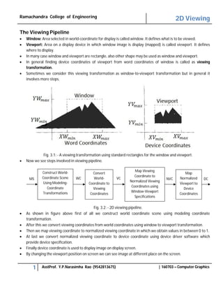
1. 2D Viewing
1 | 160703 – Computer Graphics
The Viewing Pipeline
 Window: Area selected in world-coordinate for display is called window. It defines what is to be viewed.
 Viewport: Area on a display device in which window image is display (mapped) is called viewport. It defines
where to display.
 In many case window and viewport are rectangle, also other shape may be used as window and viewport.
 In general finding device coordinates of viewport from word coordinates of window is called as viewing
transformation.
 Sometimes we consider this viewing transformation as window-to-viewport transformation but in general it
involves more steps.
Fig. 3.1: - A viewing transformation using standard rectangles for the window and viewport.
 Now we see steps involved in viewing pipeline.
Fig. 3.2: - 2D viewing pipeline.
 As shown in figure above first of all we construct world coordinate scene using modeling coordinate
transformation.
 After this we convert viewing coordinates from world coordinates using window to viewport transformation.
 Then we map viewing coordinate to normalized viewing coordinate in which we obtain values in between 0 to 1.
 At last we convert normalized viewing coordinate to device coordinate using device driver software which
provide device specification.
 Finally device coordinate is used to display image on display screen.
 By changing the viewport position on screen we can see image at different place on the screen.
DCNVCVCMS WC
Construct World-
Coordinate Scene
Using Modeling-
Coordinate
Transformations
Convert
World-
Coordinate to
Viewing
Coordinates
Map Viewing
Coordinate to
Normalized Viewing
Coordinates using
Window-Viewport
Specifications
Map
Normalized
Viewport to
Device
Coordinates
Ramachandra College of Engineering
AsstProf. Y.P.Narasimha Rao (9542813675)

2. 2D Viewing
2 | 160703 – Computer Graphics
 By changing the size of the window and viewport we can obtain zoom in and zoom out effect as per
requirement.
 Fixed size viewport and small size window gives zoom in effect, and fixed size viewport and larger window gives
zoom out effect.
 View ports are generally defines with the unit square so that graphics package are more device independent
which we call as normalized viewing coordinate.
Viewing Coordinate Reference Frame
Fig. 3.3: - A viewing-coordinate frame is moved into coincidence with the world frame in two steps: (a) translate
the viewing origin to the world origin, and then (b) rotate to align the axes of the two systems.
 We can obtain reference frame in any direction and at any position.
 For handling such condition first of all we translate reference frame origin to standard reference frame origin
and then we rotate it to align it to standard axis.
 In this way we can adjust window in any reference frame.
 this is illustrate by following transformation matrix:
M , = RT
 Where T is translation matrix and R is rotation matrix.
Window-To-Viewport Coordinate Transformation
 Mapping of window coordinate to viewport is called window to viewport transformation.
 We do this using transformation that maintains relative position of window coordinate into viewport.
 That means center coordinates in window must be remains at center position in viewport.
 We find relative position by equation as follow:
x − x
x − x
=
x − x
x − x
y − y
y − y
=
y − y
y − y
 Solving by making viewport position as subject we obtain:
x = x + (x − x )s
Ramachandra College of Engineering
AsstProf. Y.P.Narasimha Rao (9542813675)

3. 2D Viewing
3 | 160703 – Computer Graphics
y = y + (y − y )s
 Where scaling factor are :
s =
x − x
x − x
s =
y − y
y − y
 We can also map window to viewport with the set of transformation, which include following sequence of
transformations:
1. Perform a scaling transformation using a fixed-point position of (xWmin,ywmin) that scales the window area to
the size of the viewport.
2. Translate the scaled window area to the position of the viewport.
 For maintaining relative proportions we take (sx = sy). in case if both are not equal then we get stretched or
contracted in either the x or y direction when displayed on the output device.
 Characters are handle in two different way one way is simply maintain relative position like other primitive and
other is to maintain standard character size even though viewport size is enlarged or reduce.
 Number of display device can be used in application and for each we can use different window-to-viewport
transformation. This mapping is called the workstation transformation.
Fig. 3.4: - workstation transformation.
 As shown in figure two different displays devices are used and we map different window-to-viewport on each
one.
Clipping Operations
 Generally, any procedure that identifies those portions of a picture that are either inside or outside of a
specified region of space is referred to as a clipping algorithm, or simply clipping. The region against which an
object is to clip is called a clip window.
 Clip window can be general polygon or it can be curved boundary.
Application of Clipping
 It can be used for displaying particular part of the picture on display screen.
Ramachandra College of Engineering
AsstProf. Y.P.Narasimha Rao (9542813675)

4. 2D Viewing
4 | 160703 – Computer Graphics
 Identifying visible surface in 3D views.
 Antialiasing.
 Creating objects using solid-modeling procedures.
 Displaying multiple windows on same screen.
 Drawing and painting.
Point Clipping
 In point clipping we eliminate those points which are outside the clipping window and draw points which are
inside the clipping window.
 Here we consider clipping window is rectangular boundary with edge (xwmin,xwmax,ywmin,ywmax).
 So for finding wether given point is inside or outside the clipping window we use following inequality:
≤ ≤
≤ ≤
 If above both inequality is satisfied then the point is inside otherwise the point is outside the clipping window.
Line Clipping
 Line clipping involves several parts. First case is completely inside second case is completely outside and third
case include partially inside or partially outside the clipping window.
Fig. 3.5: - Line clipping against a rectangular window.
 Line which is completely inside is display completely. Line which is completely outside is eliminated from display.
And for partially inside line we need to calculate intersection with window boundary and find which part is
inside the clipping boundary and which part is eliminated.
 For line clipping several scientists tried different methods to solve this clipping procedure. Some of them are
discuss below.
Cohen-Sutherland Line Clipping
 This is one of the oldest and most popular line-clipping procedures.
P5
P1
P2
P6
P7
P8
After Clipping
(b)
Window
P5
P1
P2
P3
P4
P6
P7
P8
P9
P10
Before Clipping
(a)
Window
Ramachandra College of Engineering
AsstProf. Y.P.Narasimha Rao (9542813675)

5. 2D Viewing
5 | 160703 – Computer Graphics
 In this we divide whole space into nine region and assign 4 bit code to each endpoint of line depending on the
position where the line endpoint is located.
Fig. 3.6: - Workstation transformation.
 Figure 3.6 shows code for line end point which is fall within particular area.
 Code is deriving by setting particular bit according to position of area.
Set bit 1: For left side of clipping window.
Set bit 2: For right side of clipping window.
Set bit 3: For below clipping window.
Set bit 4: For above clipping window.
 All bits as mention above are set means 1 and other are 0.
 After assigning code we check both end points code if both endpoint have code 0000 then line is completely
inside.
 If both are not 0000 then we perform logical ending between this two code and check the result if result is non
zero line is completely outside the clipping window.
 Otherwise we calculate the intersection point with the boundary one by one and divide the line into two parts
from intersection point and perform same procedure for both line segments until we get all segments
completely inside or completely outside.
 Draw line segment which are completely inside and eliminate other line segment which found completely
outside.
 Now we discuss how to calculate intersection points with boundary.
 For intersection calculation we use line equation “ = + ”.
 For left and right boundary x coordinate is constant for left “ = ” and for right “ = ” .
 We calculate y coordinate of intersection for this boundary by putting values of x as follow:
= + ( − )
 Similarly fro top and bottom boundary y coordinate is constant for top “ = ” and for bottom “ =
”.
 We calculate x coordinate of intersection for this boundary by putting values of y as follow:
= +
−
10001001
00000001
0101 0100 0110
0010
1010
Ramachandra College of Engineering
AsstProf. Y.P.Narasimha Rao (9542813675)

6. 2D Viewing
9 | 160703 – Computer Graphics
( − )( − ) < ( − )( − )

= + ( − )
= + ( − )
 For example when we calculate intersection with left boundary x = xL, with u = (xL – x1)/ (x2 – x1), so that y can be
obtain from parametric equation as below:
= +
−
−
( − )
 Similarly for top boundary y = yT and u = (yT – y1)/(y2 – y1) , so that we can calculate x intercept as follow:
= +
−
−
( − )
Polygon Clipping
 For polygon clipping we need to modify the line clipping procedure because in line clipping we need to consider
about only line segment while in polygon clipping we need to consider the area and the new boundary of the
polygon after clipping.
Sutherland-Hodgeman Polygon Clipping
 For correctly clip a polygon we process the polygon boundary as a whole against each window edge.
 This is done by whole polygon vertices against each clip rectangle boundary one by one.
 Beginning with the initial set of polygon vertices we first clip against the left boundary and produce new
sequence of vertices.
 Then that new set of vertices is clipped against the right boundary clipper, a bttom boundary clipper and a top
boundary clipper, as shown in figure below.
Fig. 3.11: - Clipping a polygon against successive window boundaries.
Fig. 3.12: - Processing the vertices of the polygon through boundary clipper.
 There are four possible cases when processing vertices in sequence around the perimeter of a polygon.
in out
Left
Clipper
Right
Clipper
Bottom
Clipper
Top
Clipper
Ramachandra College of Engineering
AsstProf. Y.P.Narasimha Rao (9542813675)

7. 2D Viewing
10 | 160703 – Computer Graphics
Fig. 3.13: - Clipping a polygon against successive window boundaries.
 As shown in case 1: if both vertices are inside the window we add only second vertices to output list.
 In case 2: if first vertices is inside the boundary and second vertices is outside the boundary only the edge
intersection with the window boundary is added to the output vertex list.
 In case 3: if both vertices are outside the window boundary nothing is added to window boundary.
 In case 4: first vertex is outside and second vertex is inside the boundary, then adds both intersection point with
window boundary, and second vertex to the output list.
 When polygon clipping is done against one boundary then we clip against next window boundary.
 We illustrate this method by simple example.
Fig. 3.14: - Clipping a polygon against left window boundaries.
 As shown in figure above we clip against left boundary vertices 1 and 2 are found to be on the outside of the
boundary. Then we move to vertex 3, which is inside, we calculate the intersection and add both intersection
point and vertex 3 to output list.
 Then we move to vertex 4 in which vertex 3 and 4 both are inside so we add vertex 4 to output list, similarly
from 4 to 5 we add 5 to output list, then from 5 to 6 we move inside to outside so we add intersection pint to
output list and finally 6 to 1 both vertex are outside the window so we does not add anything.
 Convex polygons are correctly clipped by the Sutherland-Hodgeman algorithm but concave polygons may be
displayed with extraneous lines.
Ramachandra College of Engineering
AsstProf. Y.P.Narasimha Rao (9542813675)

8. rejected.
Step 4 − Repeat step 1 for other lines.
Cyrus-Beck Line Clipping Algorithm
This algorithm is more efficient than Cohen-Sutherland algorithm. It employs parametric line
representation and simple dot products.
Parametric equation of line is −
P0P1:P(t) = P0 + t(P1 - P0)
Let Ni be the outward normal edge Ei. Now pick any arbitrary point PEi on edge Ei then the dot
product Ni.[Pt – PEi] determines whether the point Pt is “inside the clip edge” or “outside” the clip
edge or “on” the clip edge.
The point Pt is inside if Ni.[Pt – PEi] < 0
The point Pt is outside if Ni.[Pt – PEi] > 0
The point Pt is on the edge if Ni.[Pt – PEi] = 0 Intersectionpoint
Ni.[Pt – PEi] = 0
Ni.[ P0 + t(P1 - P0) – PEi] = 0 ReplacingP(t with P0 + t(P1 - P0))
Ni.[P0 – PEi] + Ni.t[P1 - P0] = 0
Ni.[P0 – PEi] + Ni∙tD = 0 (substituting D for [P1 - P0])
Ni.[P0 – PEi] = - Ni∙tD
The equation for t becomes,
t =
Ni . [Po −PEi ]
−Ni .D
It is valid for the following conditions −
Ni ≠ 0 errorcannothappen
D!=0