Download as PDF, PPTX
![[course site]
Santiago Pascual de la Puente
santi.pascual@upc.edu
PhD Candidate
Universitat Politecnica de Catalunya
Technical University of Catalonia
Deep Generative Models I
#DLUPC](https://image.slidesharecdn.com/dlai2017d09l2-171128152227/85/Deep-Generative-Models-I-DLAI-D9L2-2017-UPC-Deep-Learning-for-Artificial-Intelligence-1-320.jpg)
![[course site]
Santiago Pascual de la Puente
santi.pascual@upc.edu
PhD Candidate
Universitat Politecnica de Catalunya
Technical University of Catalonia
Deep Generative Models I
#DLUPC](https://image.slidesharecdn.com/dlai2017d09l2-171128152227/75/Deep-Generative-Models-I-DLAI-D9L2-2017-UPC-Deep-Learning-for-Artificial-Intelligence-1-2048.jpg)

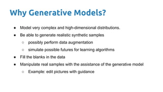
![What we are used to with Neural Nets
4
0
1
0
input
Network
output
class
Figure credit: Javier Ruiz
P(Y = [0,1,0] | X = [pixel1
, pixel2
, …, pixel784
])](https://image.slidesharecdn.com/dlai2017d09l2-171128152227/85/Deep-Generative-Models-I-DLAI-D9L2-2017-UPC-Deep-Learning-for-Artificial-Intelligence-4-320.jpg)


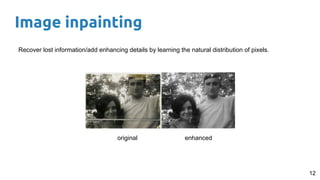
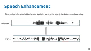
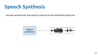
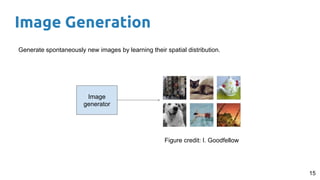
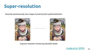


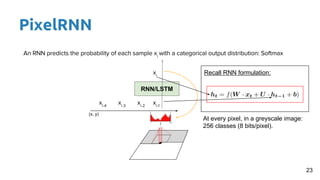


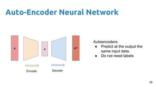
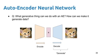


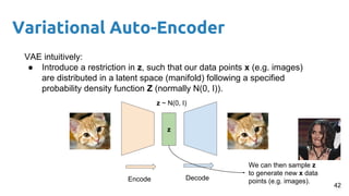
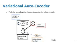
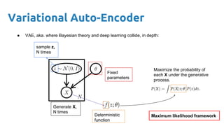


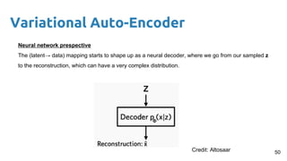


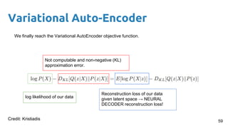


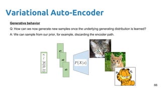


This document provides an outline and introduction to deep generative models. It discusses what generative models are, their applications like image and speech generation/enhancement, and different types of generative models including PixelRNN/CNN, variational autoencoders, and generative adversarial networks. Variational autoencoders are explained in detail, covering how they introduce a restriction in the latent space z to generate new data points by sampling from the latent prior distribution.


![제 23회 보아즈(BOAZ) 빅데이터 컨퍼런스 - [MBOAX] : ABSA를 활용한 소비자 반응 분석 기반 운영 효율화 대시보드 설계](https://cdn.slidesharecdn.com/ss_thumbnails/3-1boaz23rdconferencemboax-260203102709-9d519923-thumbnail.jpg?width=640&height=640&fit=bounds)


