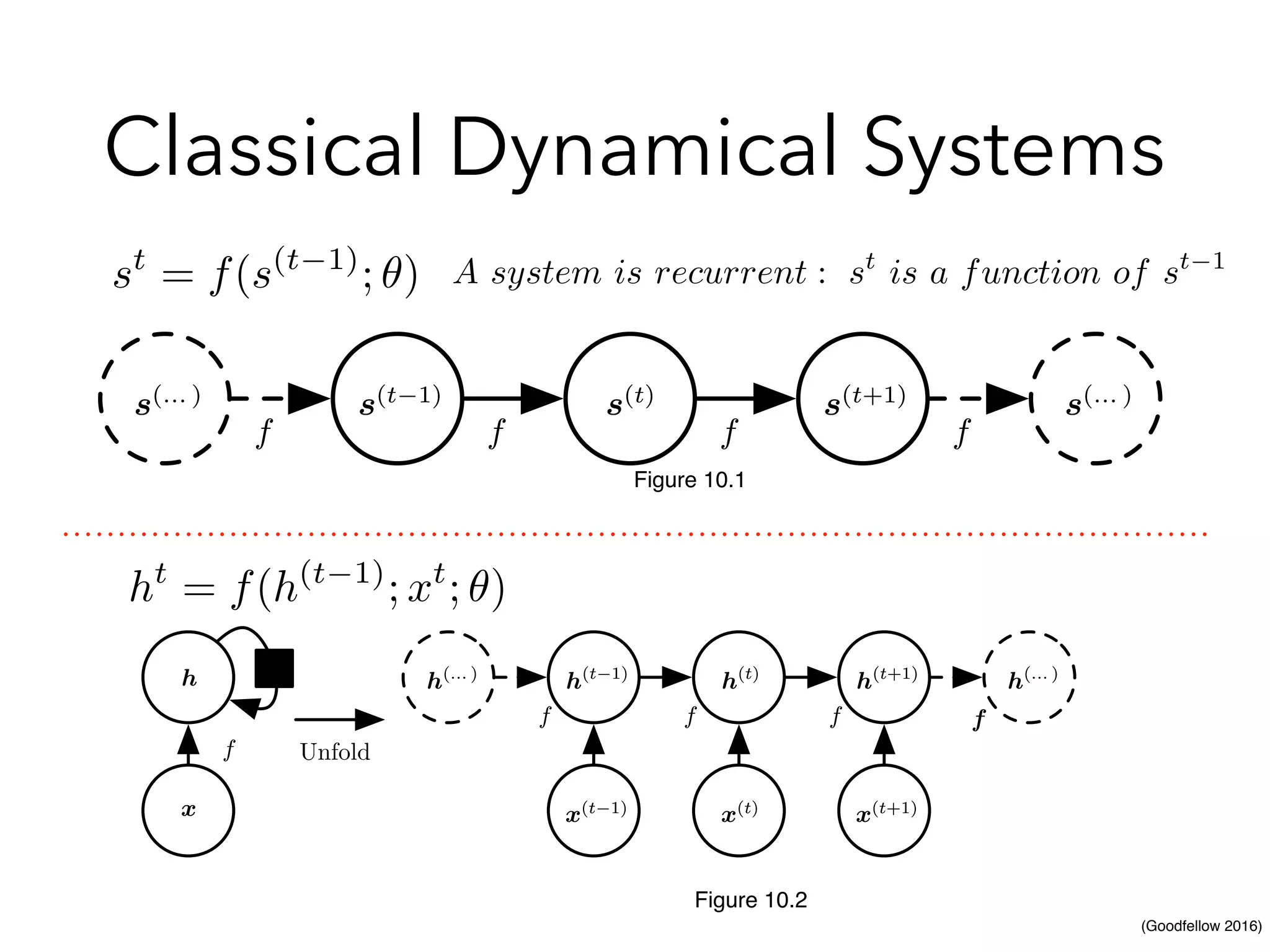
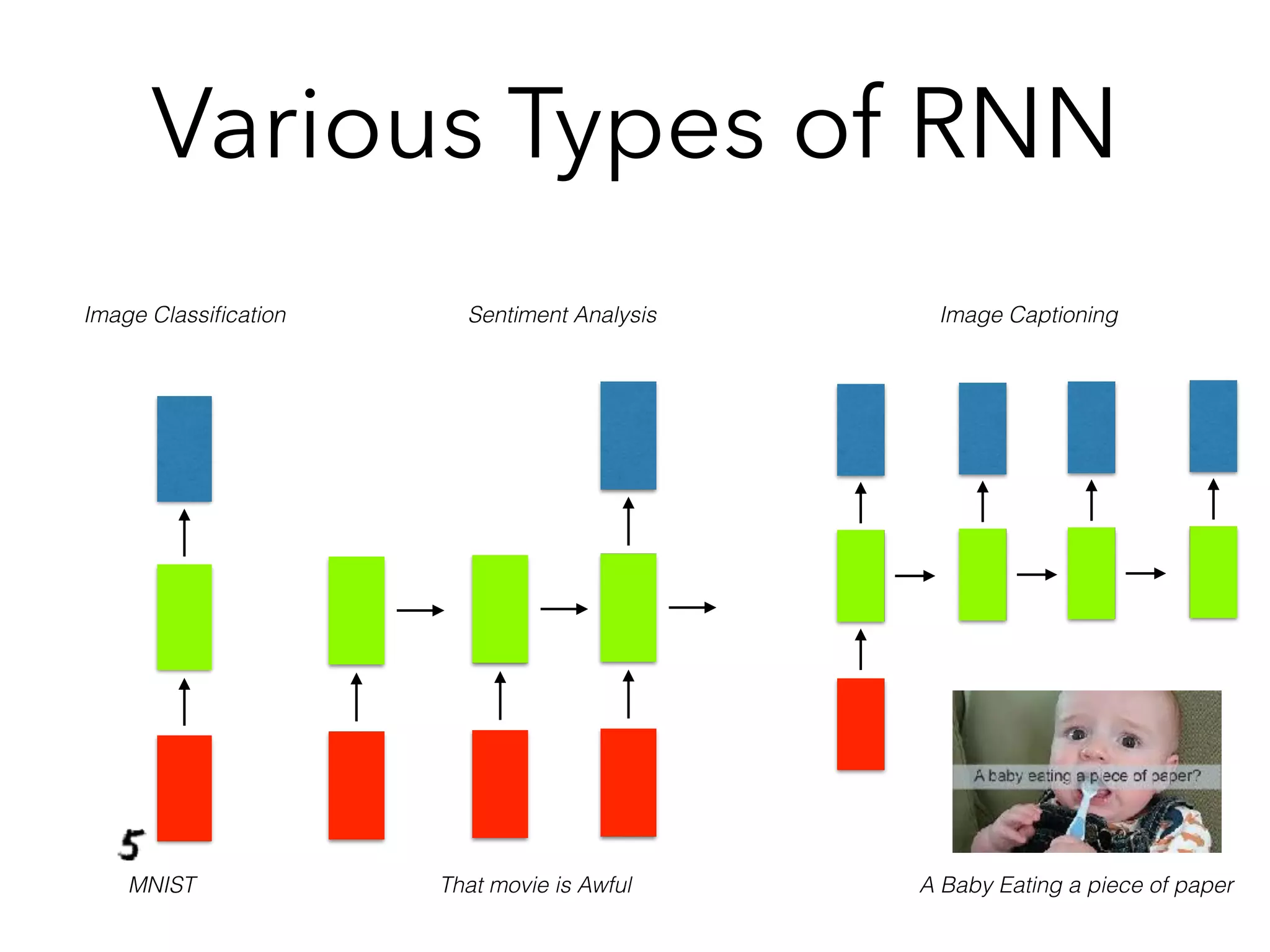
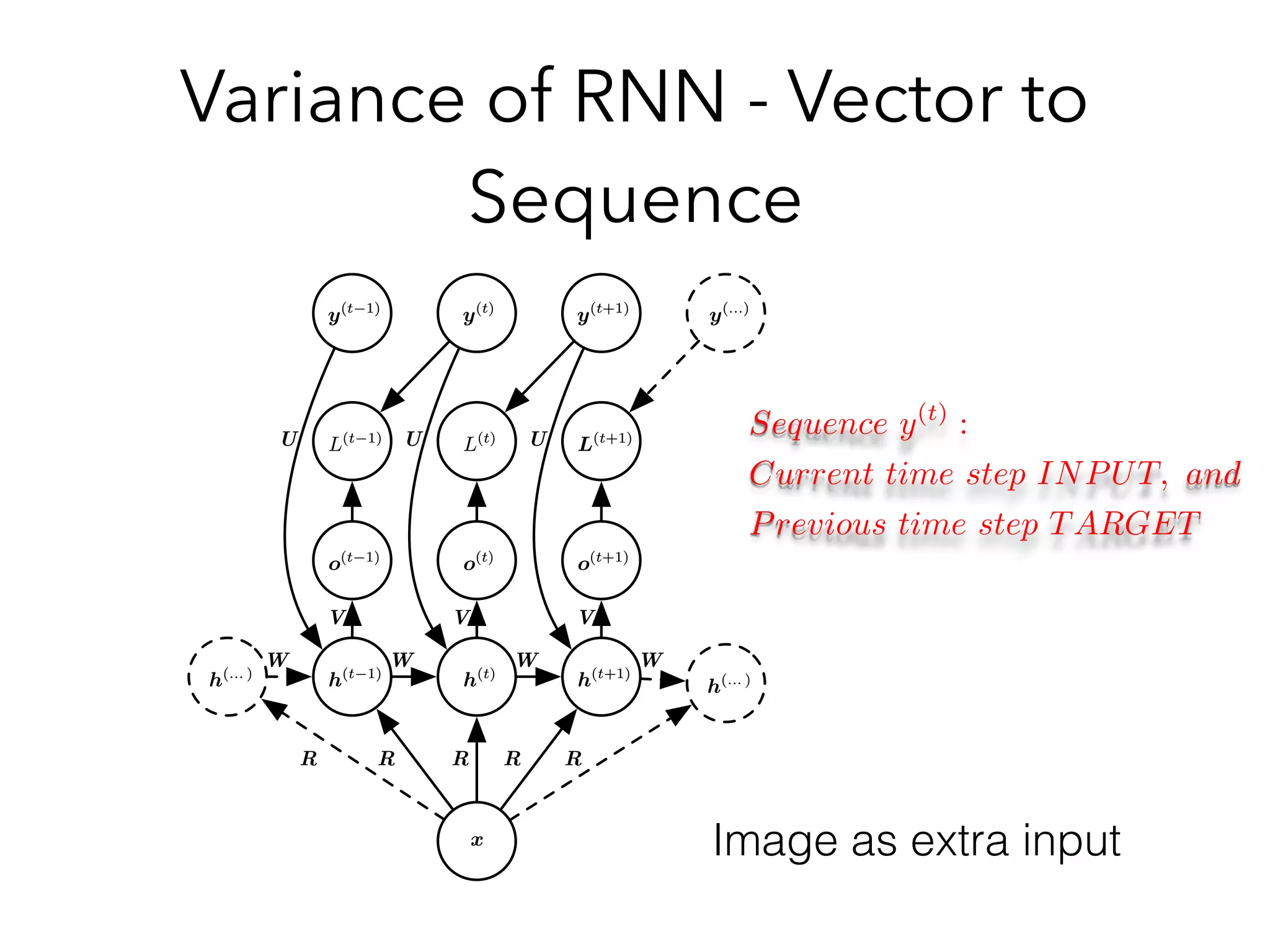
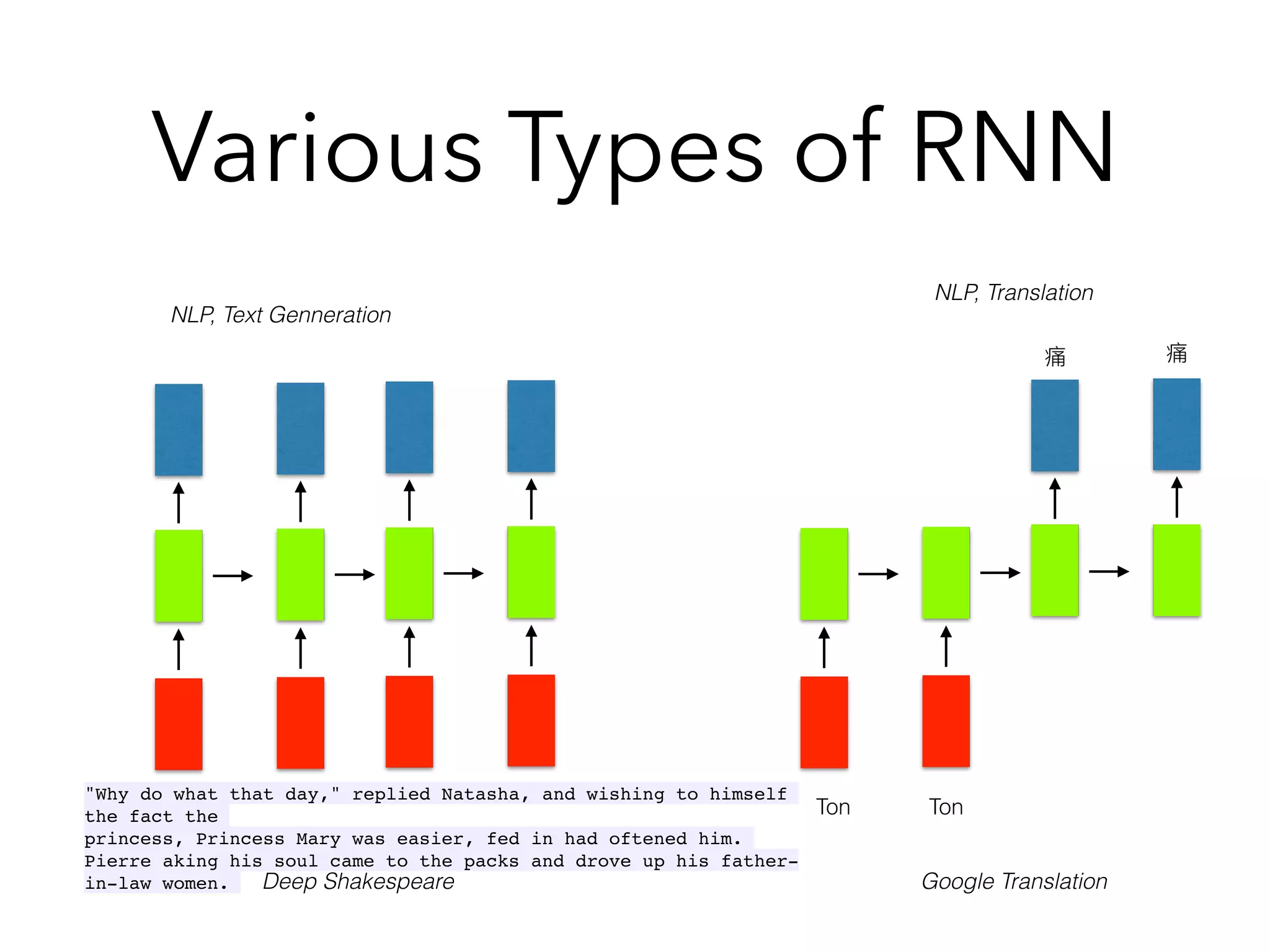
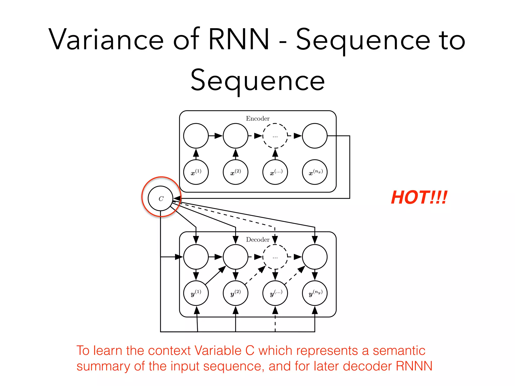
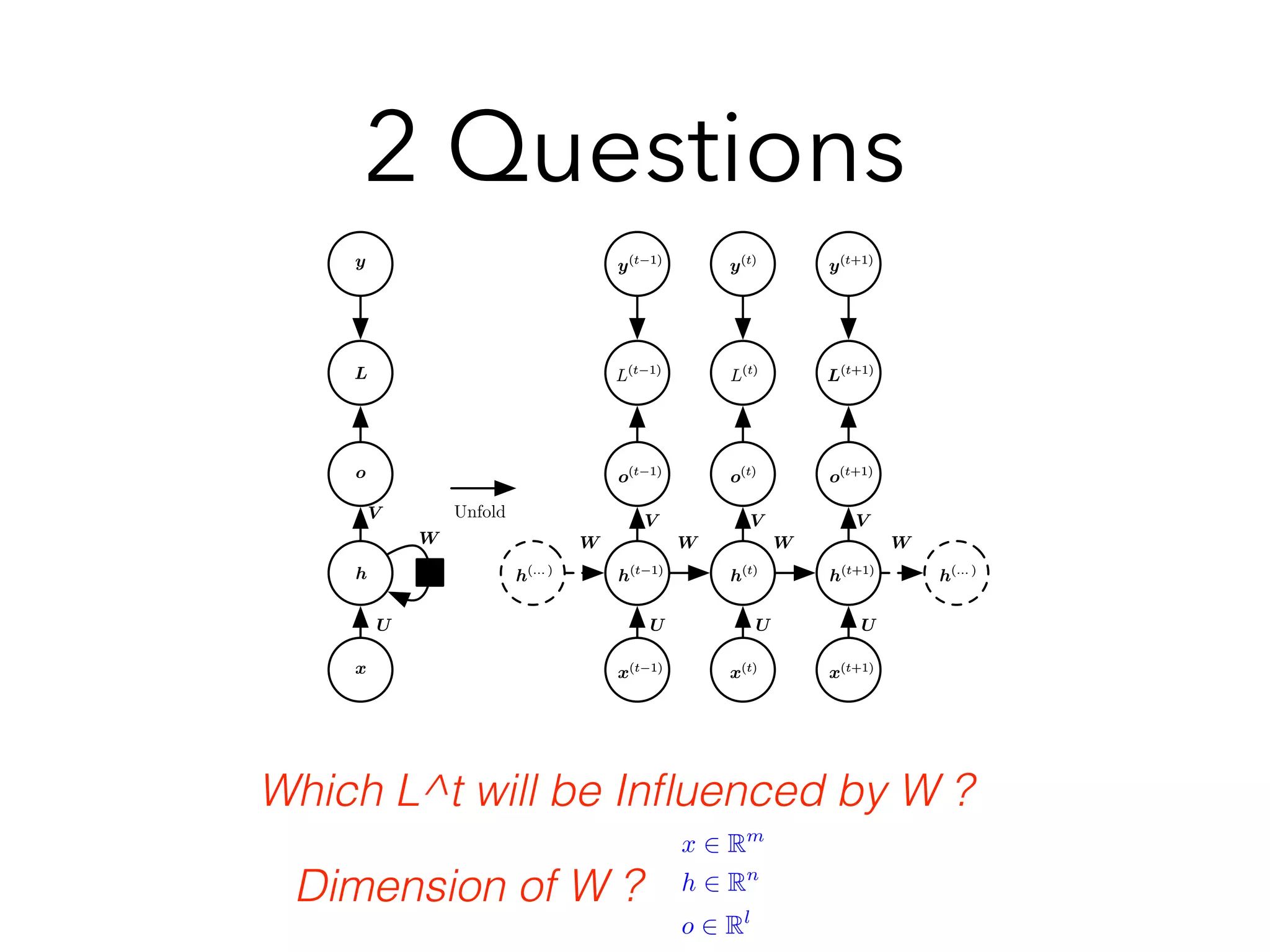
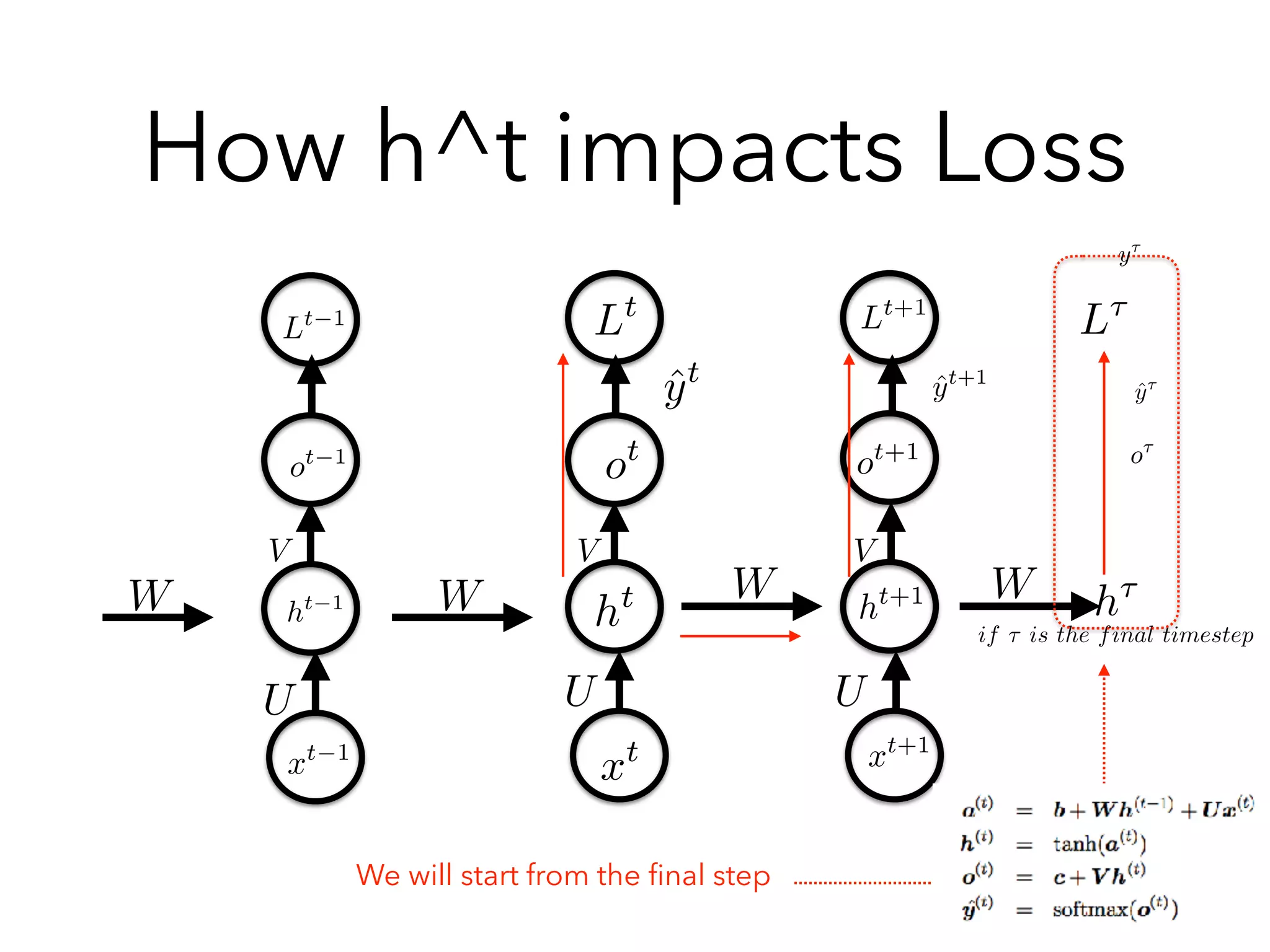
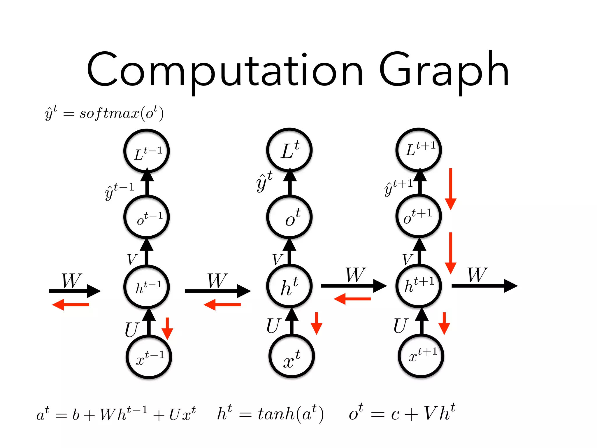
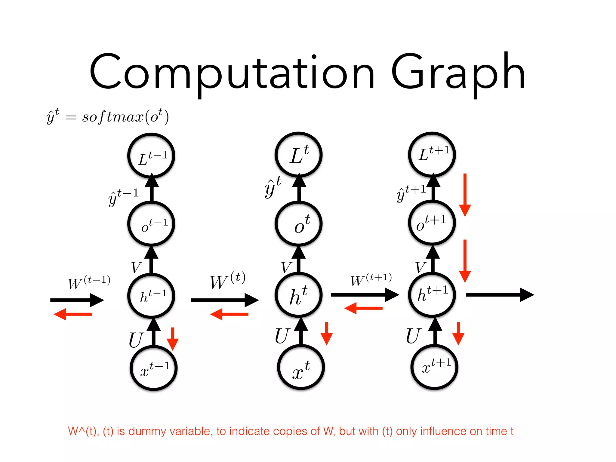
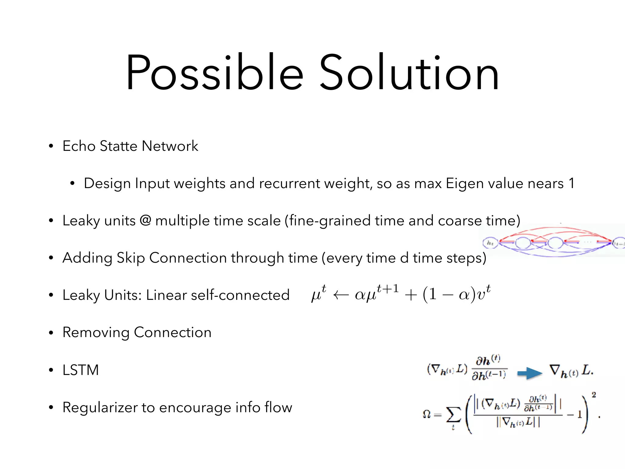
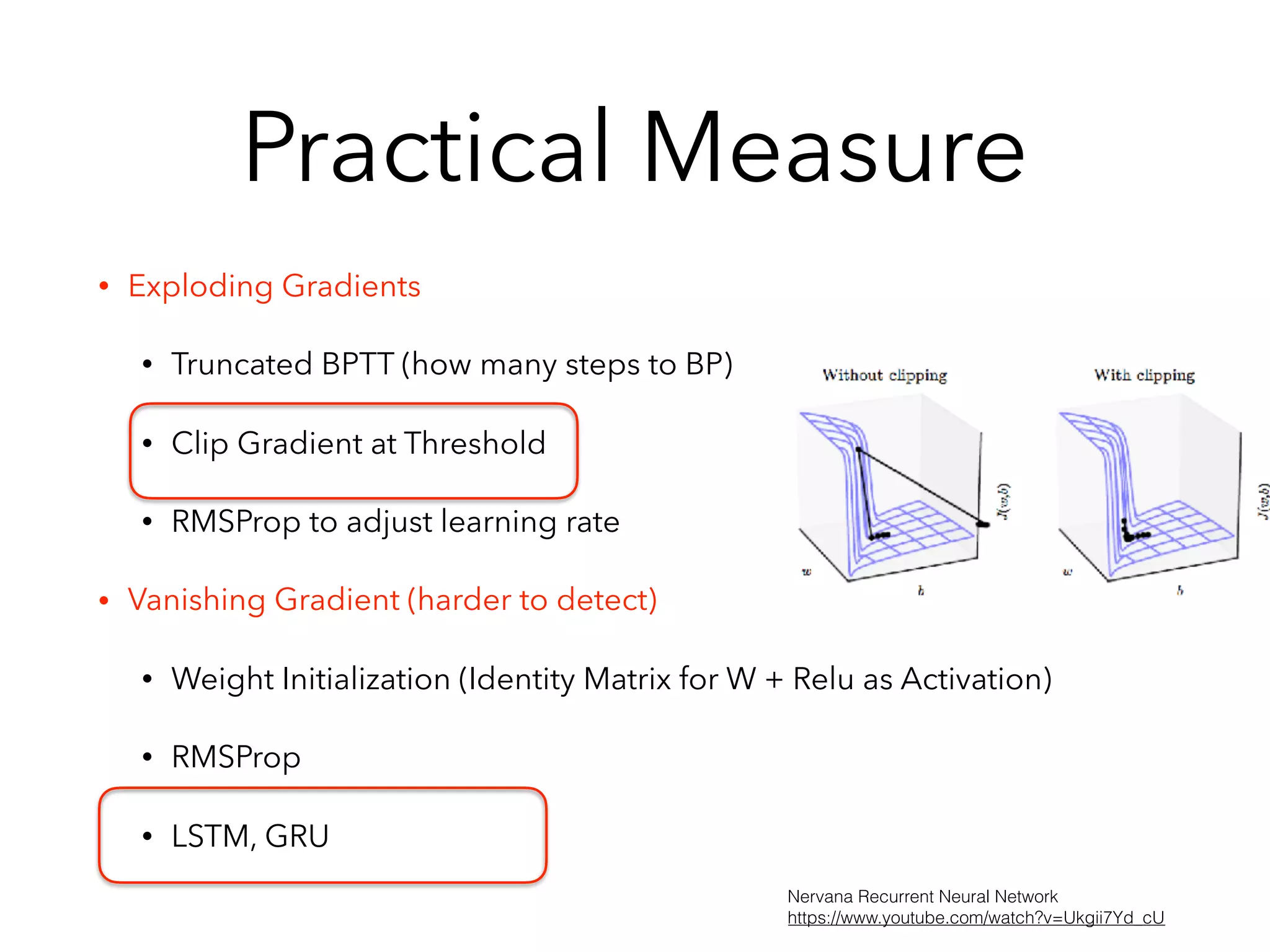
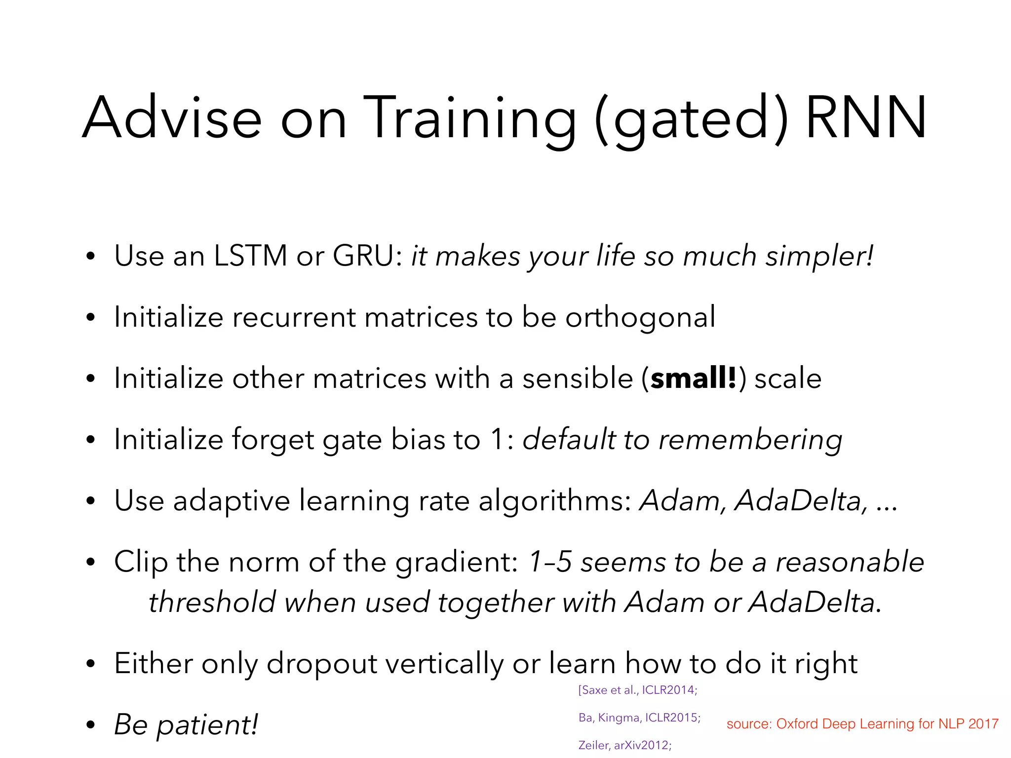
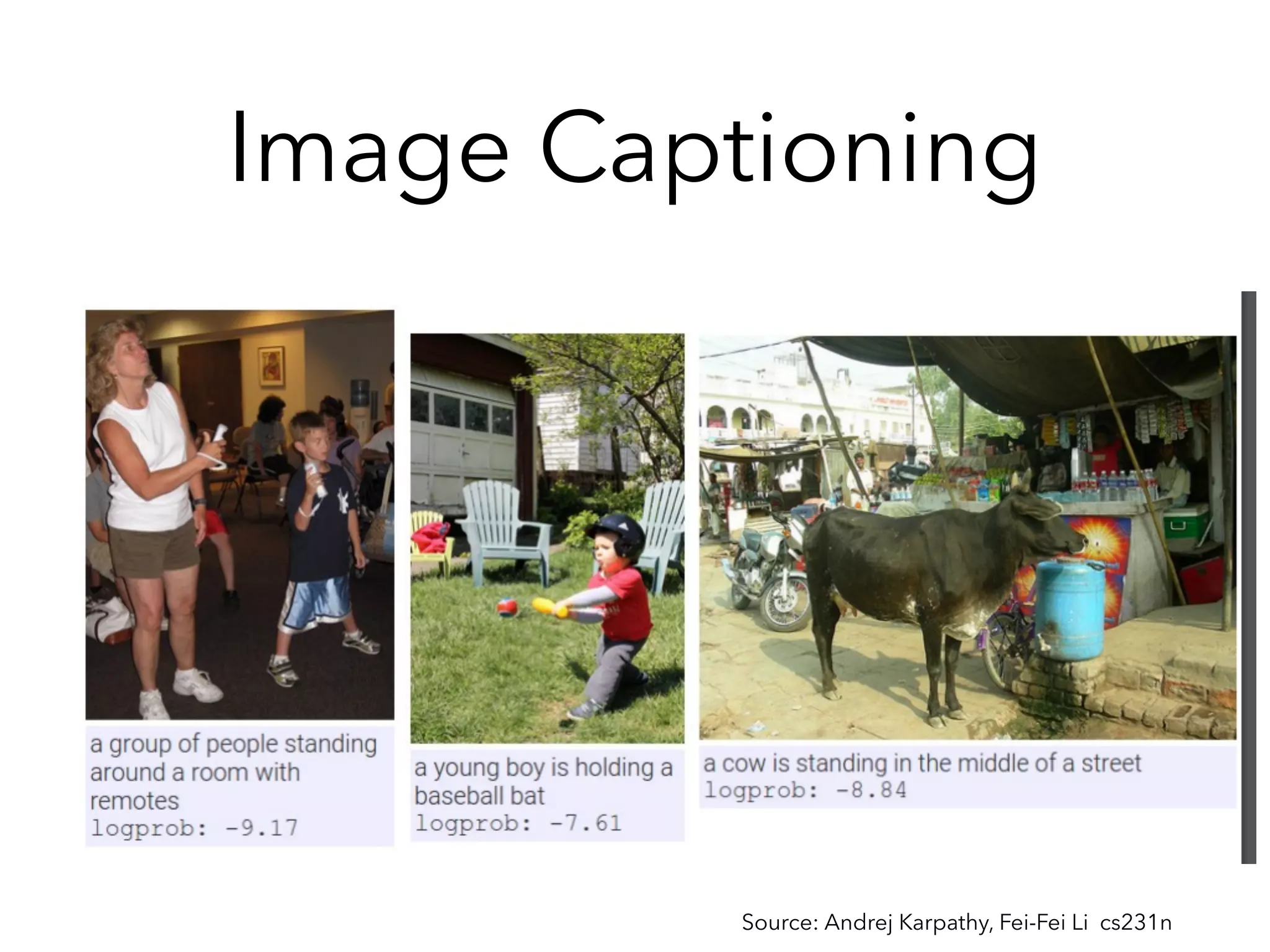
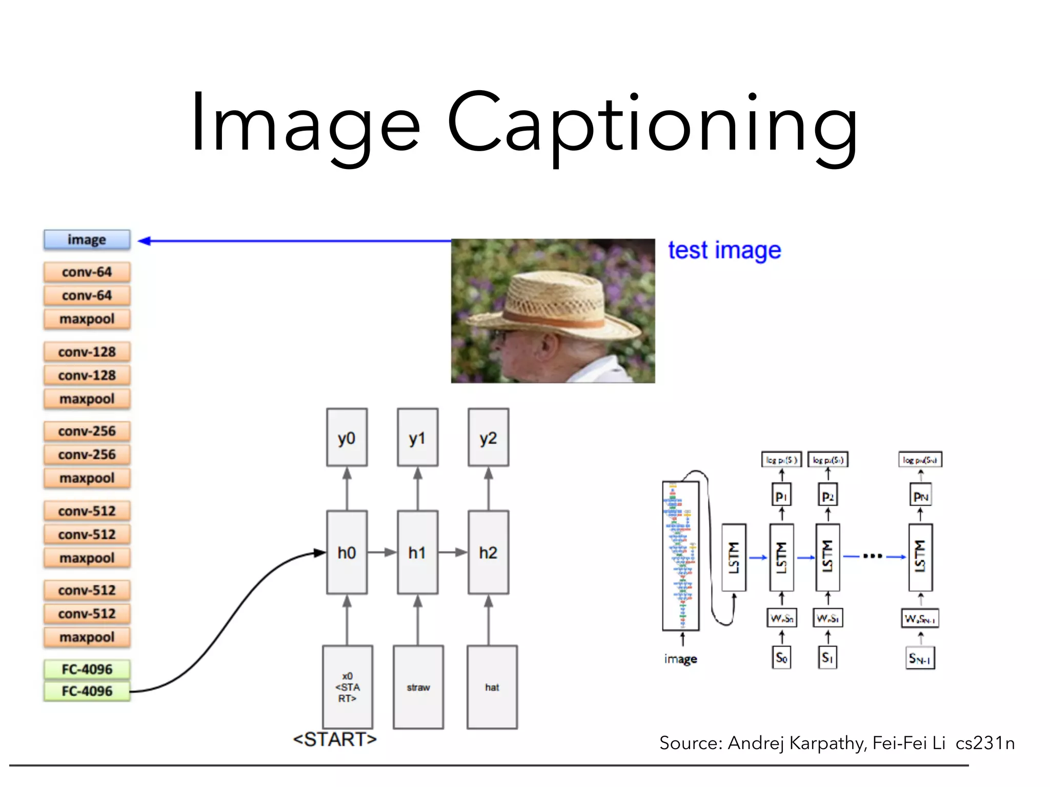
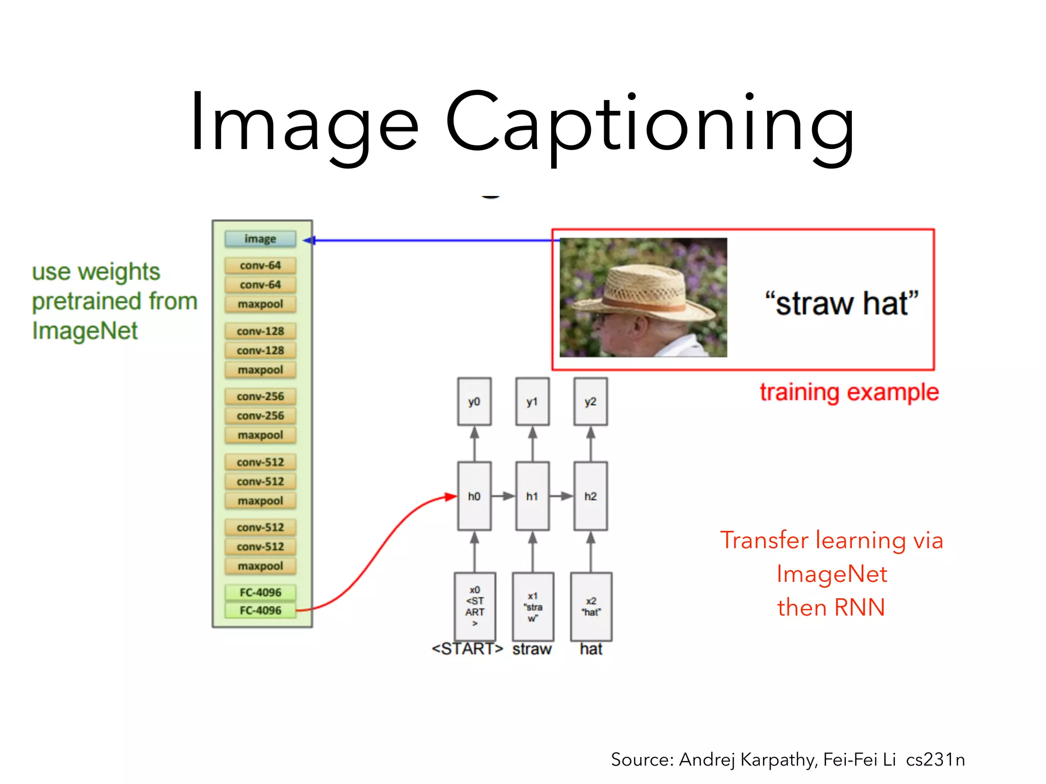
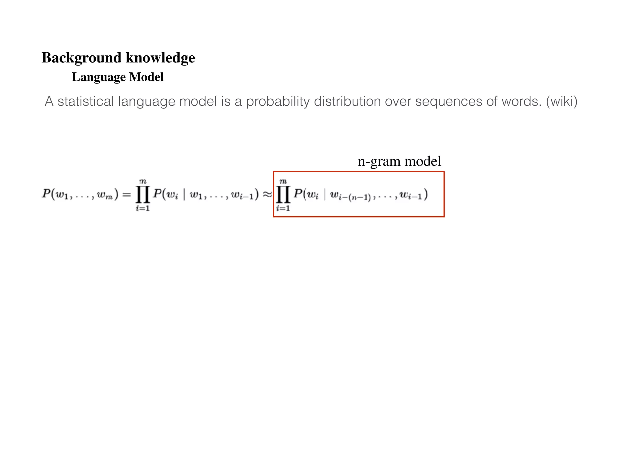
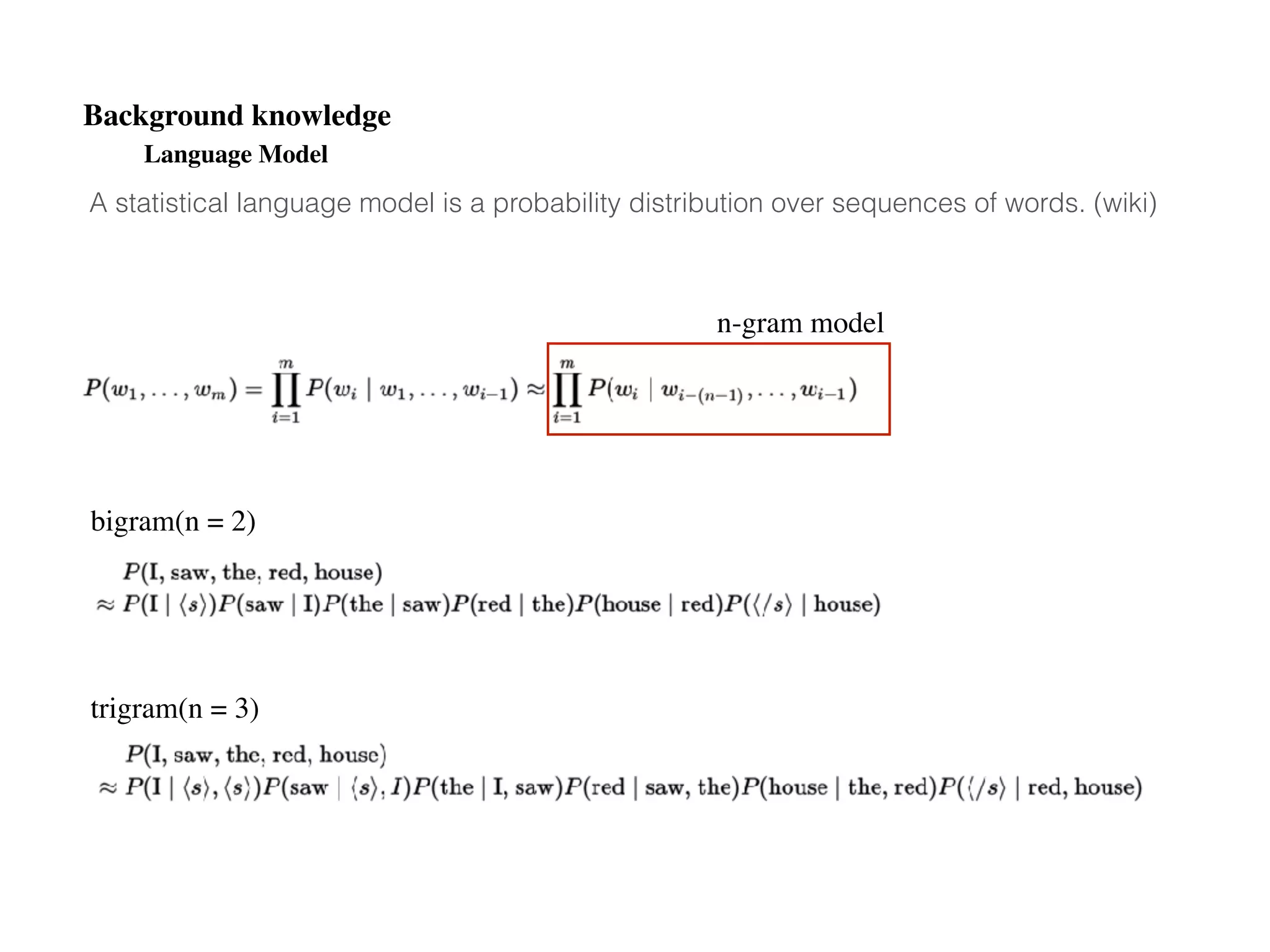
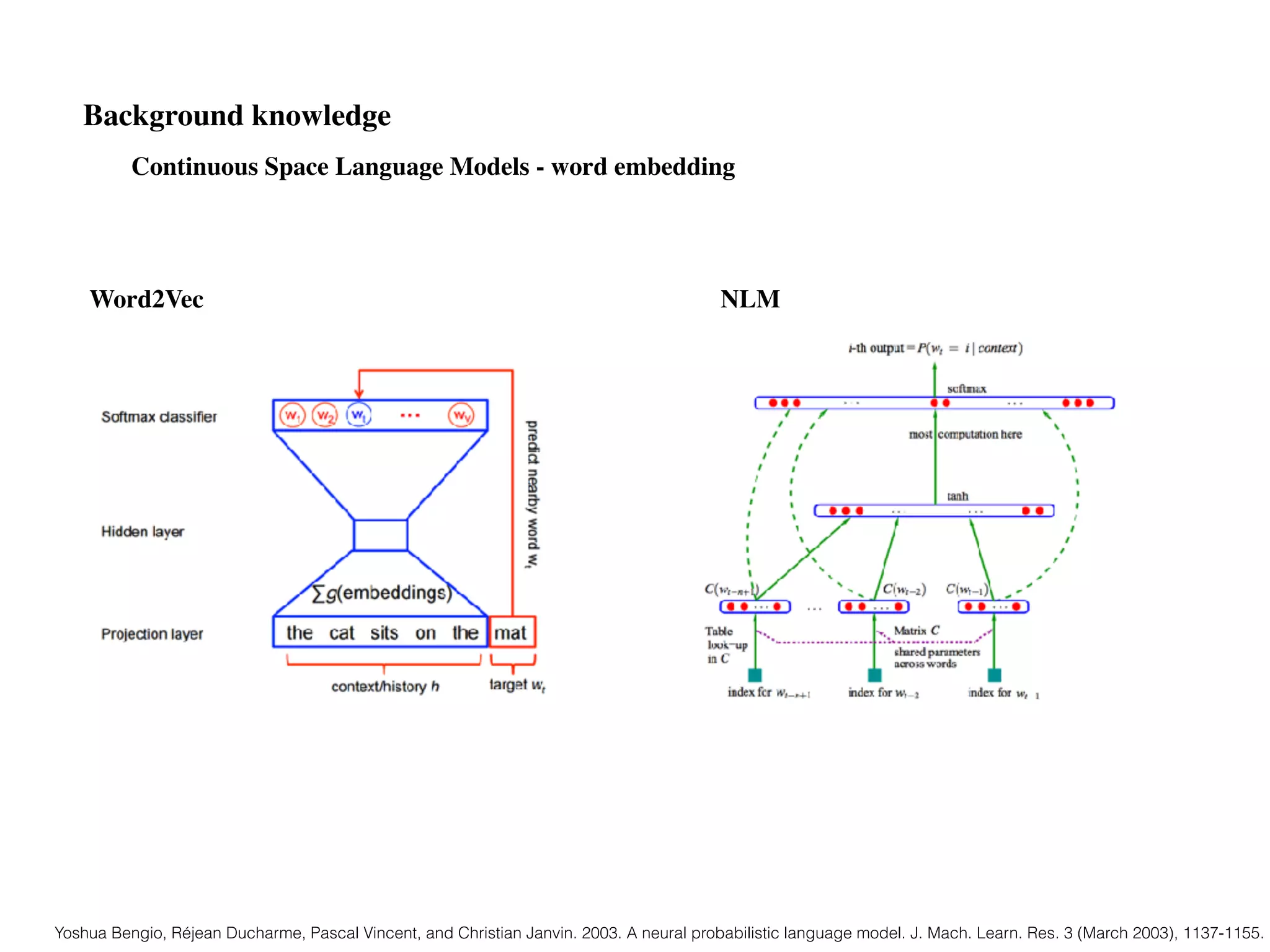
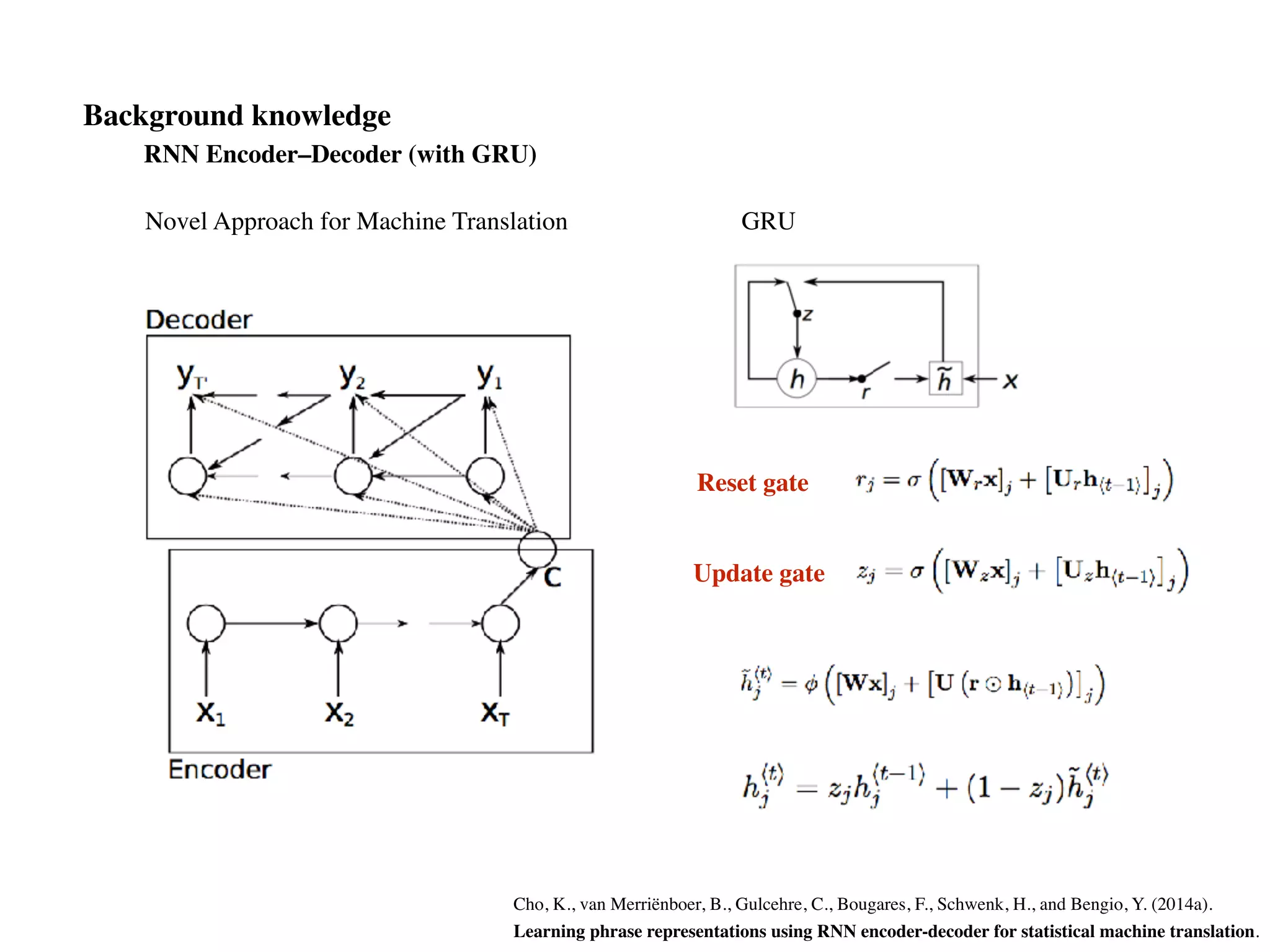
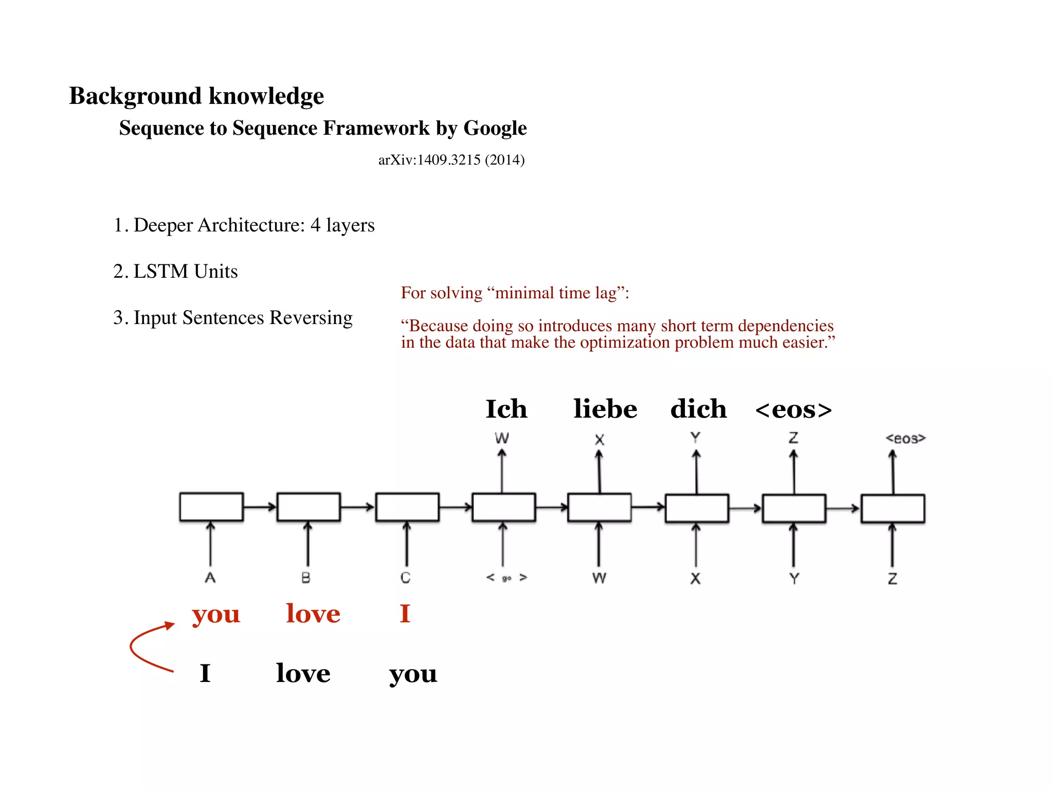
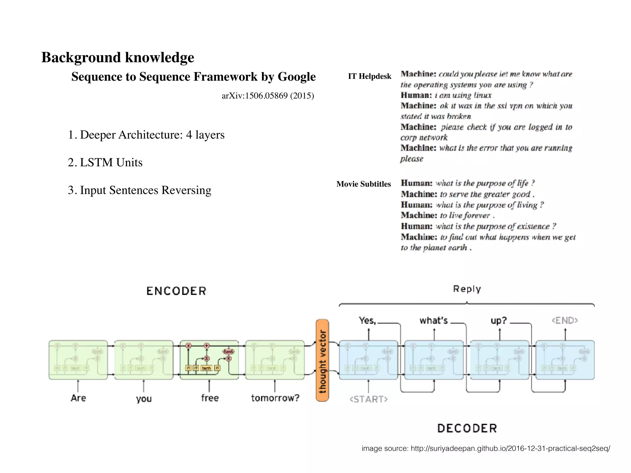
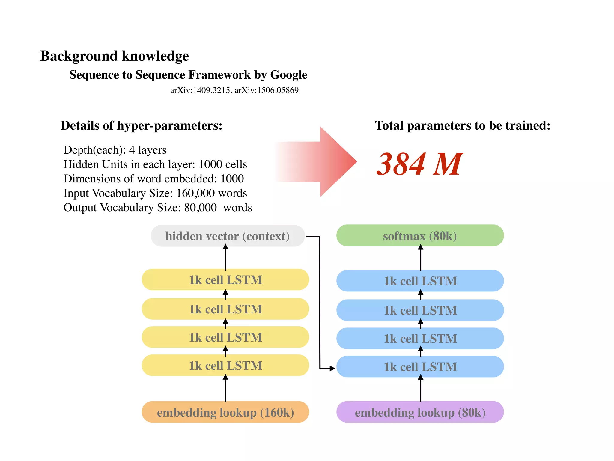
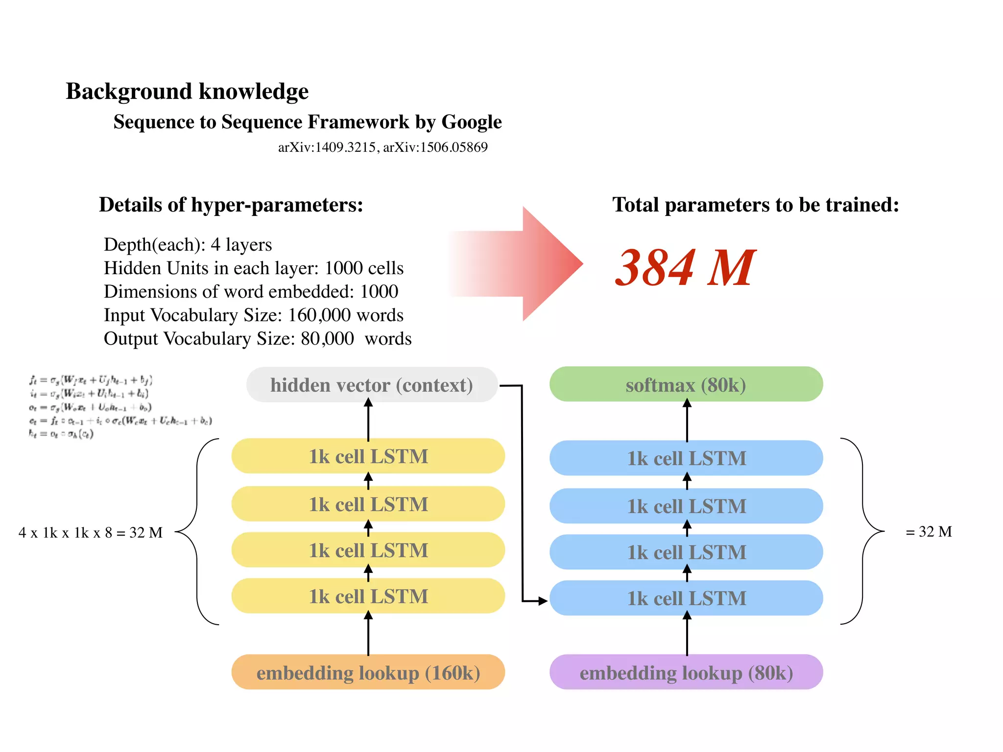
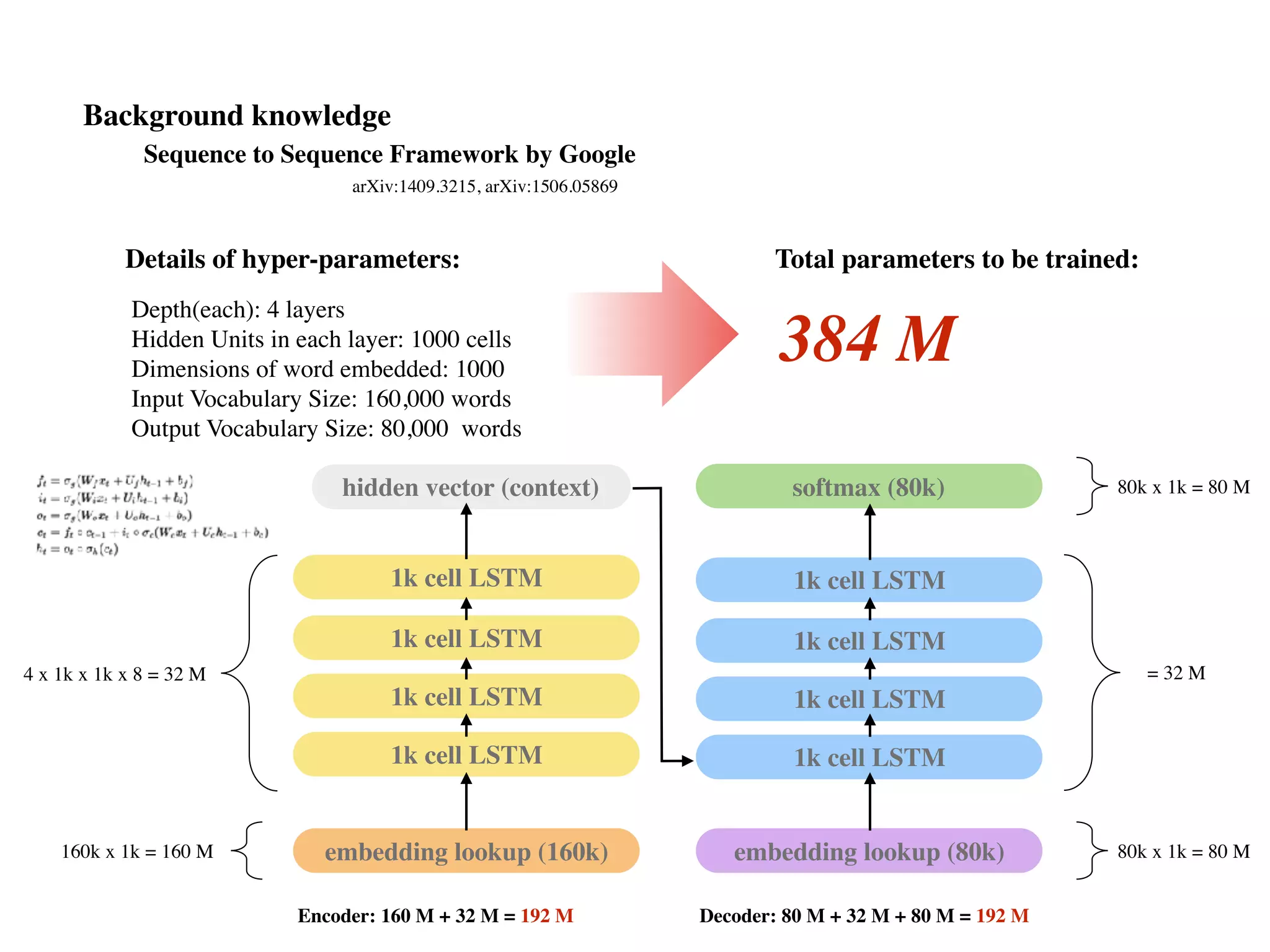
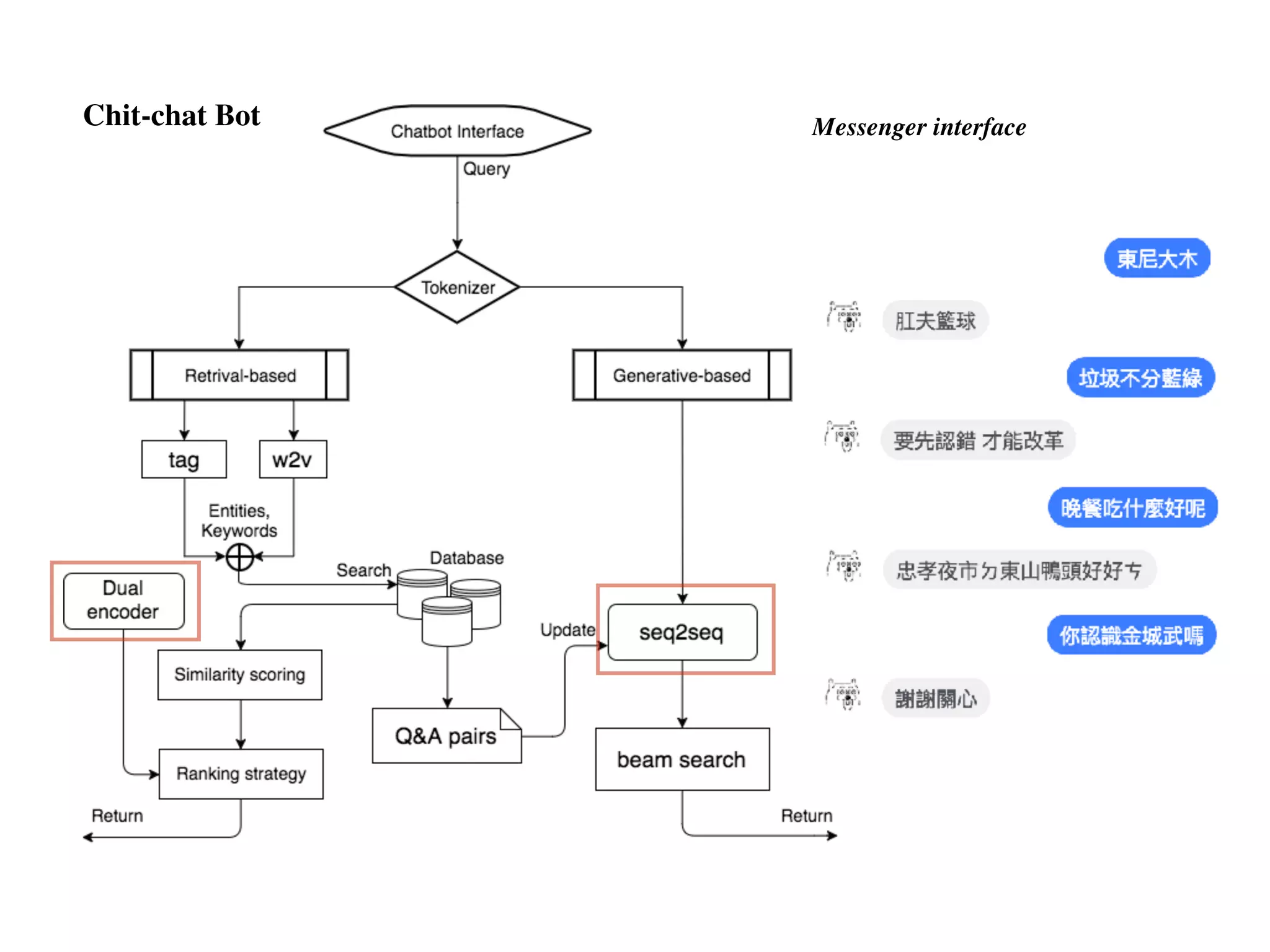
Chapter 10 discusses recurrent neural networks (RNNs), emphasizing their ability to process sequential data where order matters. It covers various types, applications, training methods like backpropagation through time (BPTT), and challenges such as exploding/vanishing gradients, introducing solutions like Long Short-Term Memory (LSTM) and Gated Recurrent Units (GRUs). The chapter also highlights practical applications of RNNs in image captioning, chatbots, and natural language processing.

1. Chapter 10: RNN
Larry Guo(tcglarry@gmail.com)
Date: May 5th, ‘17
http://www.deeplearningbook.org/

2. Agenda
• RNN Briefing
• Motivation
• Various Types &
Applications
• Train RNN -BPTT (Math!)
• Exploding/Vanishing
Gradients
• Countermeasures
• Long Short Term Memory (LSTM)
• Briefing
• GRU & Peephole
• How it helps ?
• Comparison on Various LSTM
• Real World Practice
• Image Captioning
• SVHN
• Sequence to Sequence (by Teammate
Ryan Chao)
• Chatbot(by Teammate Ryan Chao)

3. Motivation of RNN
• Sequential Data, Time Step Input(order of data matters)
• eg. This movie is good, really not bad
• vs. This movie is bad, really not good.
• Sharing Parameter across different part of model
• (Separate Parameter cannot generalize in different time steps)
• Eg. “I went to Nepal in 2009” vs “In 2009, I went to Nepal”
• 2009 is the key info we want, regardless it appears in any position

4. Using FF or CNN?
• Feed Forward
• Separate Parameter for each Input
• Needs to Learn ALL of the Rules of Languages
• CNN
• Output of CNN is a Small Number of
Neighboring Member of Inputs

5. (Goodfellow 2016)
Classical Dynamical Systems
ding the equation by repeatedly applying the definition in this
n expression that does not involve recurrence. Such an expre
epresented by a traditional directed acyclic computational gra
computational graph of equation 10.1 and equation 10.3 is illus
1.
s(t 1)
s(t 1)
s(t)
s(t)
s(t+1)
s(t+1)
ff
s(... )
s(... )
s(... )
s(... )
ff ff ff
1: The classical dynamical system described by equation 10.1, illustra
computational graph. Each node represents the state at some time
maps the state at t to the state at t + 1. The same parameters (the s
to parametrize f) are used for all time steps.
other example, let us consider a dynamical system driven by an
),
s(t)
= f(s(t 1)
, x(t)
; ✓),
Figure 10.1
st
= f(s(t 1)
; ✓)
as output layers that read information out of the state h to make predictions.
When the recurrent network is trained to perform a task that requires predicting
the future from the past, the network typically learns to use h(t) as a kind of lossy
summary of the task-relevant aspects of the past sequence of inputs up to t. This
summary is in general necessarily lossy, since it maps an arbitrary length sequence
(x(t), x(t 1), x(t 2), . . . , x(2), x(1)) to a fixed length vector h(t). Depending on the
training criterion, this summary might selectively keep some aspects of the past
sequence with more precision than other aspects. For example, if the RNN is used
in statistical language modeling, typically to predict the next word given previous
words, it may not be necessary to store all of the information in the input sequence
up to time t, but rather only enough information to predict the rest of the sentence.
The most demanding situation is when we ask h(t) to be rich enough to allow
one to approximately recover the input sequence, as in autoencoder frameworks
(chapter 14).
ff
hh
xx
h(t 1)
h(t 1)
h(t)
h(t)
h(t+1)
h(t+1)
x(t 1)
x(t 1)
x(t)
x(t)
x(t+1)
x(t+1)
h(... )
h(... )
h(... )
h(... )
ff
Unfold
ff ff f
Figure 10.2: A recurrent network with no outputs. This recurrent network just processes
ht
= f(h(t 1)
; xt
; ✓)
Figure 10.2
A system is recurrent : st
is a function of st 1

6. Recurrent Hidden Units
Input
Hidden State
Output
Loss
Target
ˆy = softmax(o)
For Every Time Step!!
Basic Form

7. (Goodfellow 2016)
Recurrent Hidden Units
information flows.
10.2 Recurrent Neural Networks
Armed with the graph unrolling and parameter sharing ideas of section 10.1, we
can design a wide variety of recurrent neural networks.
UU
VV
WW
o(t 1)
o(t 1)
hh
oo
yy
LL
xx
o(t)
o(t)
o(t+1)
o(t+1)
L(t 1)
L(t 1)
L(t)
L(t)
L(t+1)
L(t+1)
y(t 1)
y(t 1)
y(t)
y(t)
y(t+1)
y(t+1)
h(t 1)
h(t 1)
h(t)
h(t)
h(t+1)
h(t+1)
x(t 1)
x(t 1)
x(t)
x(t)
x(t+1)
x(t+1)
WWWW WW WW
h(... )
h(... )
h(... )
h(... )
VV VV VV
UU UU UU
Unfold
Figure 10.3: The computational graph to compute the training loss of a recurrent network
that maps an input sequence of x values to a corresponding sequence of output o values.
A loss L measures how far each o is from the corresponding training target y. When using
softmax outputs, we assume o is the unnormalized log probabilities. The loss L internally
Figure 10.3

8. mation flow forward in time (computing outputs and losses) and backward
me (computing gradients) by explicitly showing the path along which this
mation flows.
2 Recurrent Neural Networks
d with the graph unrolling and parameter sharing ideas of section 10.1, we
esign a wide variety of recurrent neural networks.
UU
VV
WW
o(t 1)
o(t 1)
hh
oo
yy
LL
xx
o(t)
o(t)
o(t+1)
o(t+1)
L(t 1)
L(t 1)
L(t)
L(t)
L(t+1)
L(t+1)
y(t 1)
y(t 1)
y(t)
y(t)
y(t+1)
y(t+1)
h(t 1)
h(t 1)
h(t)
h(t)
h(t+1)
h(t+1)
x(t 1)
x(t 1)
x(t)
x(t)
x(t+1)
x(t+1)
WWWW WW WW
h(... )
h(... )
h(... )
h(... )
VV VV VV
UU UU UU
Unfold
Recurrent Hidden Units

9. (Goodfellow 2016)
Recurrence through only the Output
U
V
W
o(t 1)
o(t 1)
hh
oo
yy
LL
xx
o(t)
o(t)
o(t+1)
o(t+1)
L(t 1)
L(t 1)
L(t)
L(t)
L(t+1)
L(t+1)
y(t 1)
y(t 1)
y(t)
y(t)
y(t+1)
y(t+1)
h(t 1)
h(t 1)
h(t)
h(t)
h(t+1)
h(t+1)
x(t 1)
x(t 1)
x(t)
x(t)
x(t+1)
x(t+1)
WW W W
o(... )
o(... )
h(... )
h(... )
V V V
U U U
Unfold
Figure 10.4: An RNN whose only recurrence is the feedback connection from the output
to the hidden layer. At each time step t, the input is xt, the hidden layer activations are
Less Powerful, Relies on Output to keep history…

10. Teacher Forcing
o(t 1)
o(t 1)
o(t)
o(t)
h(t 1)
h(t 1)
h(t)
h(t)
x(t 1)
x(t 1)
x(t)
x(t)
W
V V
U U
o(t 1)
o(t 1)
o(t)
o(t)
L(t 1)
L(t 1)
L(t)
L(t)
y(t 1)
y(t 1)
y(t)
y(t)
h(t 1)
h(t 1)
h(t)
h(t)
x(t 1)
x(t 1)
x(t)
x(t)
W
V V
U U
Train time Test time
Figure 10.6: Illustration of teacher forcing. Teacher forcing is a training technique that is
applicable to RNNs that have connections from their output to their hidden states at the
Easy to Train, Hard to Generalize’
Pro’s (of no recurrent h)
• Loss function could be
independently traded No
Recurrent h
• NO need BPTT
• Paralleled Trained
Con’s
• Hard to keep previous
info
• Can’t simulate TM
• Output is trained for
Target

11. Solution: Schedule Sampling
Flip Coin (p) to
decide whether to
choose y or choose o
Using Learning Curve
to decide p
from mostly choosing y
to mostly choosing o
In the beginning, we’d like the model to Learn CORRECTLY
then, Learn Robustly
Data Source: Samy Bengio, Oriol Vinyals, Navdeep Jaitly, Noam Shazeer
Google Research Mountain View, CA, USA
Better Result!!

12. Recurrent with Output Layer
Source:RNN with a Recurrent Output Layer for Learning of Naturalness

13. Various Types of RNN
Image Classification Sentiment Analysis Image Captioning
That movie is AwfulMNIST A Baby Eating a piece of paper

14. Variance of RNN - Vector to
Sequence
o(t 1)
o(t 1)
o(t)
o(t)
o(t+1)
o(t+1)
L(t 1)
L(t 1)
L(t)
L(t)
L(t+1)
L(t+1)
y(t 1)
y(t 1)
y(t)
y(t)
y(t+1)
y(t+1)
h(t 1)
h(t 1)
h(t)
h(t)
h(t+1)
h(t+1)
WW W W
h(... )
h(... )
h(... )
h(... )
V V V
U U U
xx
y(...)
y(...)
R R R R R
Sequence y(t)
:
Current time step INPUT, and
Previous time step TARGET
Image as extra input

15. Various Types of RNN
NLP, Text Genneration
Deep Shakespeare
NLP, Translation
Google Translation
"Why do what that day," replied Natasha, and wishing to himself
the fact the
princess, Princess Mary was easier, fed in had oftened him.
Pierre aking his soul came to the packs and drove up his father-
in-law women.
Ton Ton
痛 痛

16. Variance of RNN - Sequence to
Sequence
10.4 Encoder-Decoder Sequence-to-Sequence Architec-
tures
We have seen in figure 10.5 how an RNN can map an input sequence to a fixed-size
vector. We have seen in figure 10.9 how an RNN can map a fixed-size vector to a
sequence. We have seen in figures 10.3, 10.4, 10.10 and 10.11 how an RNN can
map an input sequence to an output sequence of the same length.
Encoder
…
x(1)
x(1)
x(2)
x(2)
x(...)
x(...)
x(nx)
x(nx)
Decoder
…
y(1)
y(1)
y(2)
y(2)
y(...)
y(...)
y(ny)
y(ny)
CC
Figure 10.12: Example of an encoder-decoder or sequence-to-sequence RNN architecture,
for learning to generate an output sequence (y(1)
, . . . , y(ny)
) given an input sequence
(x(1)
, x(2)
, . . . , x(nx)
). It is composed of an encoder RNN that reads the input sequence
and a decoder RNN that generates the output sequence (or computes the probability of a
To learn the context Variable C which represents a semantic
summary of the input sequence, and for later decoder RNNN
HOT!!!

17. Encode & Decode
CHAPTER 10. SEQUENCE MODELING: RECURRENT AND RECURSIVE NETS
10.4 Encoder-Decoder Sequence-to-Sequence Architec-
tures
We have seen in figure 10.5 how an RNN can map an input sequence to a fixed-size
vector. We have seen in figure 10.9 how an RNN can map a fixed-size vector to a
sequence. We have seen in figures 10.3, 10.4, 10.10 and 10.11 how an RNN can
map an input sequence to an output sequence of the same length.
Encoder
…
x(1)
x(1)
x(2)
x(2)
x(...)
x(...)
x(nx)
x(nx)
Decoder
…
y(1)
y(1)
y(2)
y(2)
y(...)
y(...)
y(ny)
y(ny)
CC
Figure 10.12: Example of an encoder-decoder or sequence-to-sequence RNN architecture,
這是⼀一本書 !
This is a book!

18. CHAPTER 10. SEQUENCE MODELING: RECURRENT AND RECURSIVE NETS
sequence still has one restriction, which is that the length of both sequences must
be the same. We describe how to remove this restriction in section 10.4.
o(t 1)
o(t 1)
o(t)
o(t)
o(t+1)
o(t+1)
L(t 1)
L(t 1)
L(t)
L(t)
L(t+1)
L(t+1)
y(t 1)
y(t 1)
y(t)
y(t)
y(t+1)
y(t+1)
h(t 1)
h(t 1)
h(t)
h(t)
h(t+1)
h(t+1)
x(t 1)
x(t 1)
x(t)
x(t)
x(t+1)
x(t+1)
g(t 1)
g(t 1)
g(t)
g(t)
g(t+1)
g(t+1)
Bidirectional RNN
In many cases, you have to listen till the end to get the real meaning
Some times, in NLP, using reverse input to train!

19. Bidirectional
PTER 10. SEQUENCE MODELING: RECURRENT AND RECURSIVE NETS
ence still has one restriction, which is that the length of both sequences must
he same. We describe how to remove this restriction in section 10.4.
o(t 1)
o(t 1)
o(t)
o(t)
o(t+1)
o(t+1)
L(t 1)
L(t 1)
L(t)
L(t)
L(t+1)
L(t+1)
y(t 1)
y(t 1)
y(t)
y(t)
y(t+1)
y(t+1)
h(t 1)
h(t 1)
h(t)
h(t)
h(t+1)
h(t+1)
x(t 1)
x(t 1)
x(t)
x(t)
x(t+1)
x(t+1)
g(t 1)
g(t 1)
g(t)
g(t)
g(t+1)
g(t+1)
e 10.11: Computation of a typical bidirectional recurrent neural network, meant
arn to map input sequences x to target sequences y, with loss L(t)
at each step t.
h recurrence propagates information forward in time (towards the right) while the
urrence propagates information backward in time (towards the left). Thus at each
Useful in speech recognition

20. Bidirectional RNN:
Alternative to CNN
source:ReNet: A Recurrent Neural Network Based Alternative to Convolutional Networks
Bidirectional RNN*2 (left, right top, bottom)

21. Recursive Network
be mitigated by introducing skip connections in the hidden-to-hidden path, as
rated in figure 10.13c.
6 Recursive Neural Networks
x(1)
x(1)
x(2)
x(2)
x(3)
x(3)
V V V
yy
LL
x(4)
x(4)
V
oo
U W U W
U
W
e 10.14: A recursive network has a computational graph that generalizes that of the
rent network from a chain to a tree. A variable-size sequence x(1)
, x(2)
, . . . , x(t)
can
deep learning not bad V (0
not0
) + V (0
bad0
) 6= V (0
not0
,0
bad0
)
x1 x2 x3 x4
h1
h2
h3
Recursive network is a
generalized
form of Recurrent network
Also could apply to Image Parsing
Syntax Parsing

22. (Goodfellow 2016)
Deep RNNs
h
y
x
z
(a) (b) (c)
x
h
y
x
h
y
Figure 10.13: A recurrent neural network can be made deep in many ways (Pascanu
Figure 10.13
Input to Hidden
Hidden to Hidden
Hidden to Output

23. Training RNN

24. Loss Function
information flow forward in time (computing outputs and losses) and backward
in time (computing gradients) by explicitly showing the path along which this
information flows.
10.2 Recurrent Neural Networks
Armed with the graph unrolling and parameter sharing ideas of section 10.1, we
can design a wide variety of recurrent neural networks.
UU
VV
WW
o(t 1)
o(t 1)
hh
oo
yy
LL
xx
o(t)
o(t)
o(t+1)
o(t+1)
L(t 1)
L(t 1)
L(t)
L(t)
L(t+1)
L(t+1)
y(t 1)
y(t 1)
y(t)
y(t)
y(t+1)
y(t+1)
h(t 1)
h(t 1)
h(t)
h(t)
h(t+1)
h(t+1)
x(t 1)
x(t 1)
x(t)
x(t)
x(t+1)
x(t+1)
WWWW WW WW
h(... )
h(... )
h(... )
h(... )
VV VV VV
UU UU UU
Unfold
Figure 10.3: The computational graph to compute the training loss of a recurrent network
that maps an input sequence of x values to a corresponding sequence of output o values.
A loss L measures how far each o is from the corresponding training target y. When using
softmax outputs, we assume o is the unnormalized log probabilities. The loss L internally
computes ˆy = softmax(o) and compares this to the target y. The RNN has input to hidden
+ + L =
X
t
L(t)
Initial State
Input
Hidden State
Output
Loss
Target
Negative Log Likelihood
or
Cross Entropy
Note : Need to calculate gradient of b, c, W, U, V

25. 2 Questions
Which L^t will be Influenced by W ?
Dimension of W ?
x 2 Rm
h 2 Rn
o 2 Rl
information flows.
10.2 Recurrent Neural Networks
Armed with the graph unrolling and parameter sharing ideas of section 10.1, we
can design a wide variety of recurrent neural networks.
UU
VV
WW
o(t 1)
o(t 1)
hh
oo
yy
LL
xx
o(t)
o(t)
o(t+1)
o(t+1)
L(t 1)
L(t 1)
L(t)
L(t)
L(t+1)
L(t+1)
y(t 1)
y(t 1)
y(t)
y(t)
y(t+1)
y(t+1)
h(t 1)
h(t 1)
h(t)
h(t)
h(t+1)
h(t+1)
x(t 1)
x(t 1)
x(t)
x(t)
x(t+1)
x(t+1)
WWWW WW WW
h(... )
h(... )
h(... )
h(... )
VV VV VV
UU UU UU
Unfold
Figure 10.3: The computational graph to compute the training loss of a recurrent network
that maps an input sequence of x values to a corresponding sequence of output o values.
A loss L measures how far each o is from the corresponding training target y. When using
softmax outputs, we assume o is the unnormalized log probabilities. The loss L internally
computes ˆy = softmax(o) and compares this to the target y. The RNN has input to hidden
connections parametrized by a weight matrix U, hidden-to-hidden recurrent connections
parametrized by a weight matrix W , and hidden-to-output connections parametrized by
a weight matrix V . Equation 10.8 defines forward propagation in this model. (Left)The

26. Key : Sharing Weight
in time (computing gradients) by explicitly showing the path along which this
information flows.
10.2 Recurrent Neural Networks
Armed with the graph unrolling and parameter sharing ideas of section 10.1, we
can design a wide variety of recurrent neural networks.
UU
VV
WW
o(t 1)
o(t 1)
hh
oo
yy
LL
xx
o(t)
o(t)
o(t+1)
o(t+1)
L(t 1)
L(t 1)
L(t)
L(t)
L(t+1)
L(t+1)
y(t 1)
y(t 1)
y(t)
y(t)
y(t+1)
y(t+1)
h(t 1)
h(t 1)
h(t)
h(t)
h(t+1)
h(t+1)
x(t 1)
x(t 1)
x(t)
x(t)
x(t+1)
x(t+1)
WWWW WW WW
h(... )
h(... )
h(... )
h(... )
VV VV VV
UU UU UU
Unfold
Figure 10.3: The computational graph to compute the training loss of a recurrent network
that maps an input sequence of x values to a corresponding sequence of output o values.
A loss L measures how far each o is from the corresponding training target y. When using
softmax outputs, we assume o is the unnormalized log probabilities. The loss L internally
computes ˆy = softmax(o) and compares this to the target y. The RNN has input to hidden
connections parametrized by a weight matrix U, hidden-to-hidden recurrent connections
parametrized by a weight matrix W , and hidden-to-output connections parametrized by
Share Same weight
W
Share Same weight U

27. Computation Graph
htht 1 ht+1
ot+1
ot 1
ot
Lt
Lt 1 Lt+1
xt+1
xt 1
xt
WW W W
U U U
V VV
at
= b + Wht 1
+ Uxt
ht
= tanh(at
) ot
= c + V ht
ˆyt
= softmax(ot
)
ˆyt
ˆyt 1 ˆyt+1
at
i = b +
X
j
Wijht 1
j + Uxt
at
Find Gradient!

28. Computation Graph
htht 1 ht+1
ot+1
ot 1
ot
Lt
Lt 1 Lt+1
xt+1
xt 1
xt
U U U
V VV
ˆyt
= softmax(ot
)
ˆyt
ˆyt 1 ˆyt+1
W(t 1) W(t+1)
W(t)
W^(t), (t) is dummy variable, to indicate copies of W, but with (t) only influence on time t

29. To Update Parameter
rV L =
X
t
(rot L)(ht
)T
rcL =
X
t
(rot L)
rW L =
X
t
@L
@W(t)
=
X
t
diag(1 (ht
)2
)(rht L)(ht 1
)T
rU L =
X
t
diag(1 (ht
)2
)(rht L)(xt
)T
rbL =
X
t
diag(1 (ht
)2
)(rht L)
(1), & (3) Known via Forward pass
(1)
(2)
Equation 10.26
(3)
Have to do
a. Calculate (rht L)
b. Prove equation 10.26
Wij = Wij ⌘ ⇤
@L
@Wij

30. How h^t impacts Loss
htht 1 ht+1
ot+1
ot 1
ot
Lt
Lt 1 Lt+1
xt+1
xt 1
xt
WW W W
U U U
V VV
L⌧
h⌧
if ⌧ is the final timestep
We will start from the final step
o⌧
ˆyt ˆyt+1
ˆy⌧
y⌧

31. Note : ith column of V = ith row of V T
@L
@h⌧
= rh⌧ L = V T
ro⌧ L⌧
@L
@h⌧
=
2
6
6
6
6
6
6
6
4
@L
@h⌧
1
@L
@h⌧
2
.
@L
@h⌧
i
.
.
3
7
7
7
7
7
7
7
5
@L
@h⌧
i
=
X
j
@L
@o⌧
j
@o⌧
j
@h⌧
i
=
X
j
@L
@o⌧
j
Vji =
X
j
@L
@o⌧
j
V T
ij =
⇥
V T
i1 V T
i2 . V T
ij . .
⇤
2
6
6
6
6
6
6
6
4
@L
@o⌧
1
@L
@o⌧
2
.
@L
@o⌧
j
.
.
3
7
7
7
7
7
7
7
5
when t = ⌧
= ˆyt
i 1i,y(t) = ˆyt
yt
rot Lt
rh⌧ L
ot
i = c +
X
j
Vijht
j

32. ˆyj =
eoj
P
k eok
Note :
X
j
ˆy = 1
@Lt
@ot
i
=
X
k
yt
k
@log(ˆyt
k)
@ot
i
=
X
k
yt
k
ˆyt
k
@ˆyt
k
@ot
i
=
yt
i
ˆyt
i
ˆyt
i(1 ˆyt
i)
X
k6=i
yt
k
ˆyt
k
( ˆyt
i ˆyt
k)
@ˆyt
j
@ot
i
=ˆyt
i (1 ˆyt
i ) if i = j
= ˆyt
i ˆyt
j if i 6= j
Source: http://math.stackexchange.com/questions/945871/
derivative-of-softmax-loss-function
= yt
i + ˆyt
i (
X
k
ˆyt
k) = ˆyt
yt
= yt
i + ˆyt
i ˆyt
i +
X
k6=i
yt
k ˆyt
k
Sum=1
Lt
=
X
k
yt
klog(ˆyt
k)
rot Lt
= ˆyt
i 1i,y(t)
softmax derivative

33. htht 1 ht+1
ot+1
ot 1
ot
Lt
Lt 1 Lt+1
xt+1
xt 1
xt
WW W W
U U U
V VV
for t < ⌧
rht L
at+1

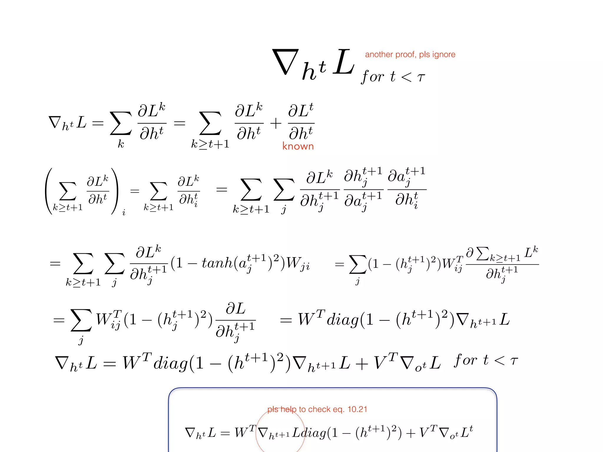
34. rht L = (
@ht+1
@ht
)T @L
@ht+1
+ (
@ot
@ht
)T @L
@ot
= V T
rot Lt
=
2
6
6
6
6
4
W11, W21, ., ., Wj1, Wn1
W12, W22, ., ., Wj2, Wn2
., ., ., ., ., .
., ., ., ., ., .
W1n, W2n, ., ., Wjn, Wnn
3
7
7
7
7
5
2
6
6
6
6
6
6
4
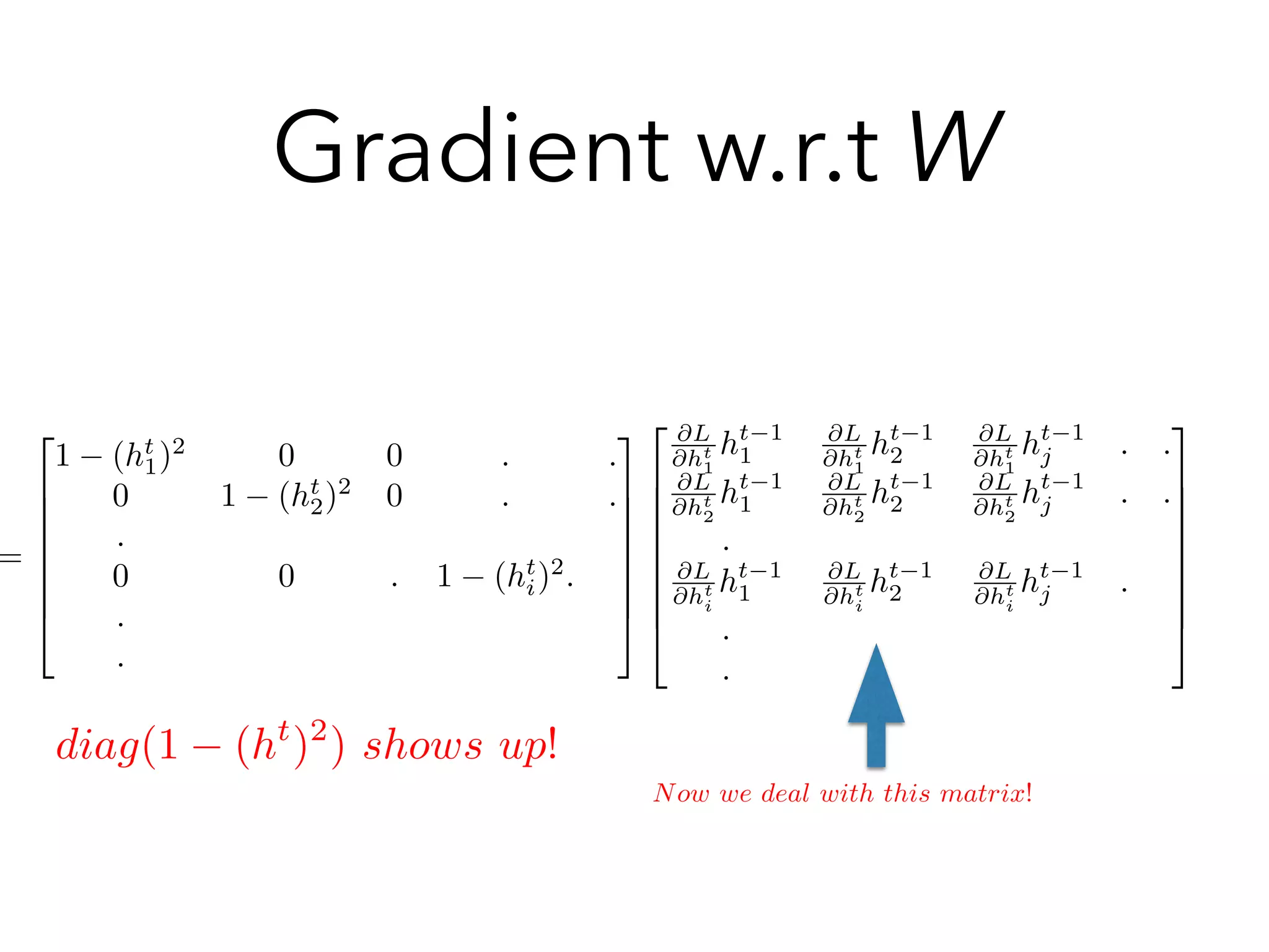
1 tan(ht
1)2
0 0 . .
0 1 tan(ht
2)2
0 . .
.
0 0 . 1 tan(ht
j)2
.
.
.
3
7
7
7
7
7
7
5
2
6
6
6
6
6
6
6
6
4
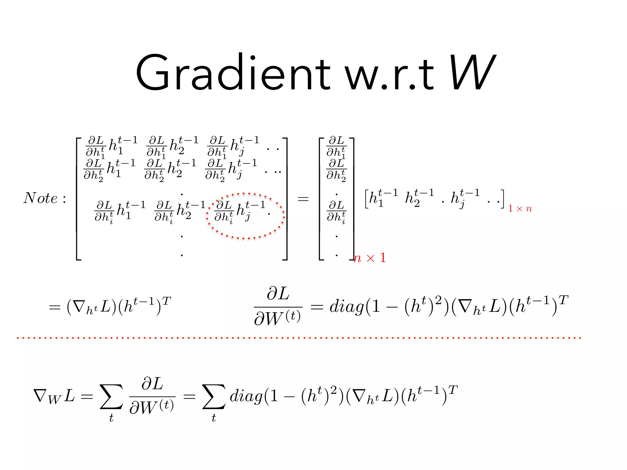
@L
@ht+1
1
@L
@ht+1
2
.
@L
@ht+1
j
.
.
3
7
7
7
7
7
7
7
7
5
(
@ht+1
@ht
)T @L
@ht+1 = WT
diag(1 (ht+1
)2
)rht+1 L
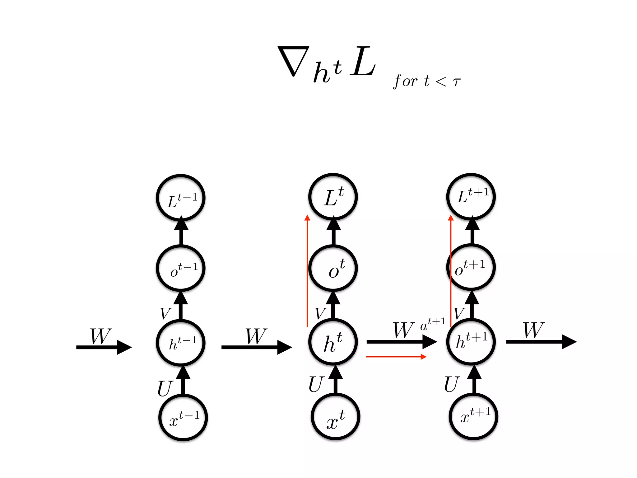
for t < ⌧
rht L Note: different to the text book
To be verified!!!!!!!!!!!
Jacobian [
@ht+1
i
@ht
j
] =
@ht+1
i
@at+1
i
·
@at+1
i
@ht
j
= Wij
@ht+1
i
@at+1
i
= Wij(1 tanh2
(at+1
i )) = diag(1 tanh2
(at+1
))W
= diag(1 (ht+1
)2
)W
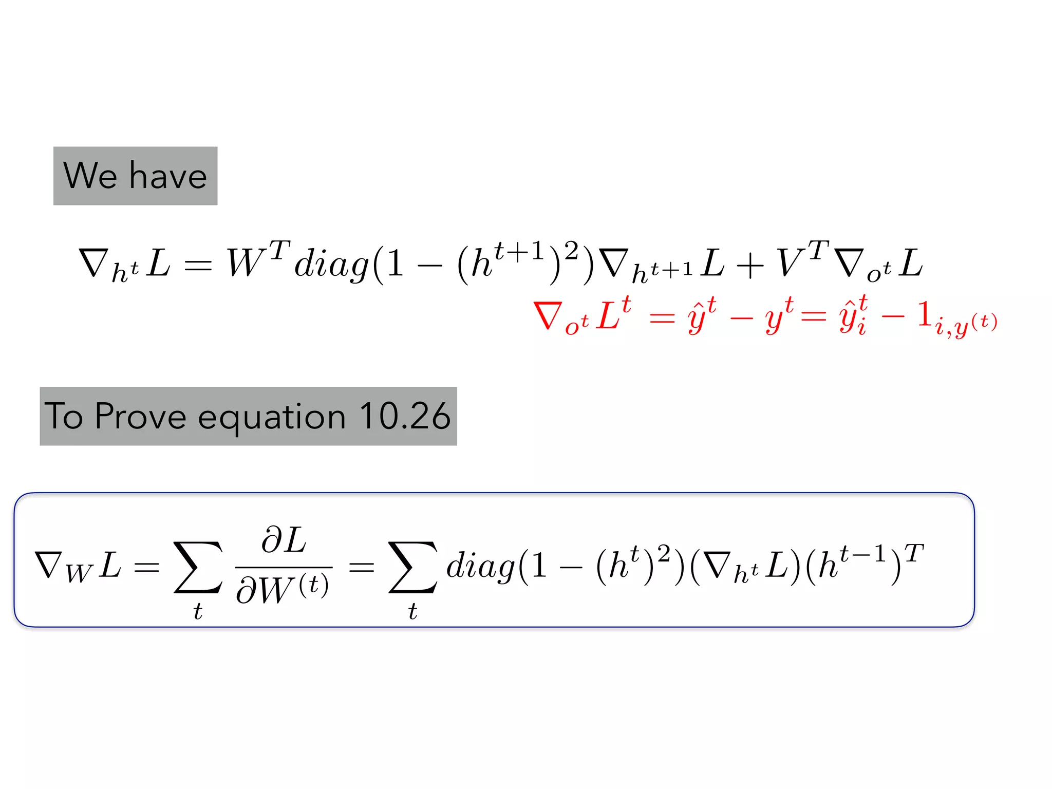
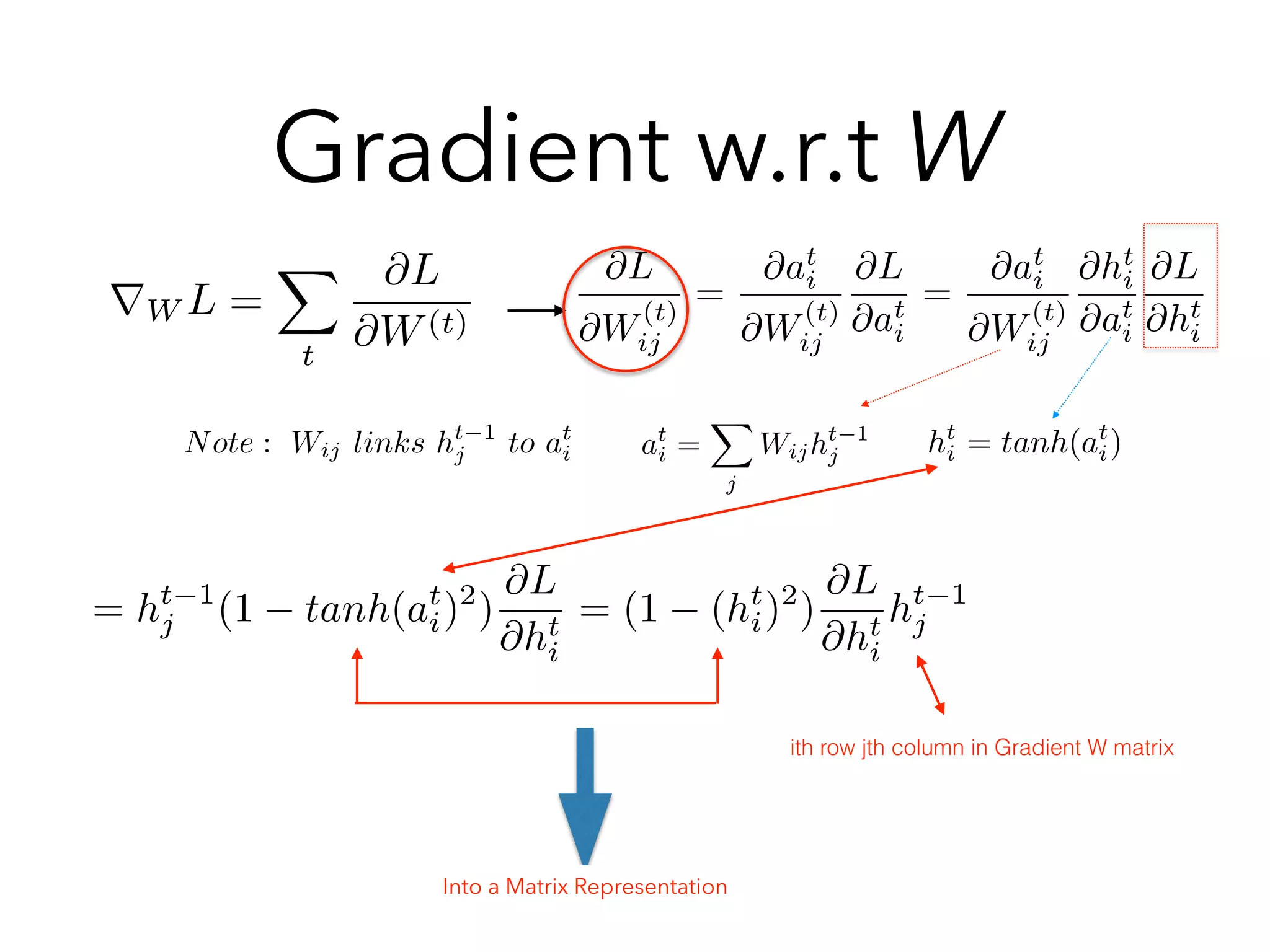
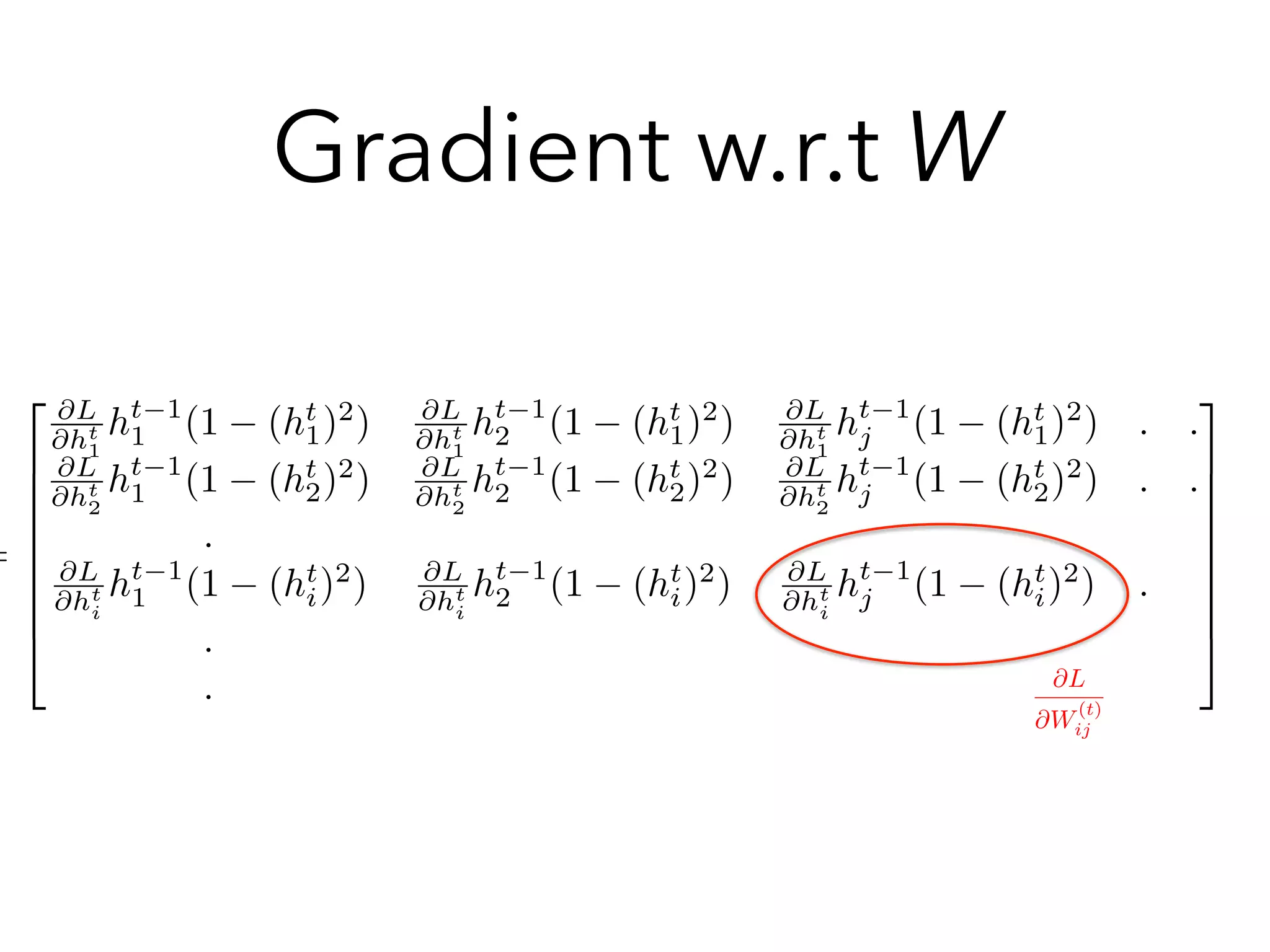
rht L = WT
rht+1 Ldiag(1 (ht+1
)2
) + V T
rot Lt
pls help to check eq. 10.21

35. for t < ⌧
rht L = WT
rht+1 Ldiag(1 (ht+1
)2
) + V T
rot Lt
pls help to check eq. 10.21
for t < ⌧
rht L
known
0
@
X
k t+1
@Lk
@ht
1
A
i
=
X
k t+1
@Lk
@ht
i
=
X
k t+1
X
j
@Lk
@ht+1
j
@ht+1
j
@at+1
j
@at+1
j
@ht
i
=
X
k t+1
X
j
@Lk
@ht+1
j
(1 tanh(at+1
j )2
)Wji =
X
j
(1 (ht+1
j )2
)WT
ij
@
P
k t+1 Lk
@ht+1
j
=
X
j
WT
ij (1 (ht+1
j )2
)
@L
@ht+1
j
rht L =
X
k
@Lk
@ht
=
X
k t+1
@Lk
@ht
+
@Lt
@ht
= WT
diag(1 (ht+1
)2
)rht+1 L
rht L = WT
diag(1 (ht+1
)2
)rht+1 L + V T
rot L
another proof, pls ignore

36. rW L =
X
t
@L
@W(t)
=
X
t
diag(1 (ht
)2
)(rht L)(ht 1
)T
To Prove equation 10.26
rht L = WT
diag(1 (ht+1
)2
)rht+1 L + V T
rot L
= ˆyt
i 1i,y(t)= ˆyt
yt
rot Lt
We have

37. Gradient w.r.t W
rW L =
X
t
@L
@W(t)
Note : Wij links ht 1
j to at
i at
i =
X
j
Wijht 1
j
@L
@W
(t)
ij
=
@at
i
@W
(t)
ij
@L
@at
i
=
@at
i
@W
(t)
ij
@ht
i
@at
i
@L
@ht
i
ht
i = tanh(at
i)
= ht 1
j (1 tanh(at
i)2
)
@L
@ht
i
= (1 (ht
i)2
)
@L
@ht
i
ht 1
j
Into a Matrix Representation
ith row jth column in Gradient W matrix

38. @L
@W
(t)
ij
=
2
6
6
6
6
6
6
6
4
@L
@ht
1
ht 1
1 (1 (ht
1)2
) @L
@ht
1
ht 1
2 (1 (ht
1)2
) @L
@ht
1
ht 1
j (1 (ht
1)2
) . .
@L
@ht
2
ht 1
1 (1 (ht
2)2
) @L
@ht
2
ht 1
2 (1 (ht
2)2
) @L
@ht
2
ht 1
j (1 (ht
2)2
) . .
.
@L
@ht
i
ht 1
1 (1 (ht
i)2
) @L
@ht
i
ht 1
2 (1 (ht
i)2
) @L
@ht
i
ht 1
j (1 (ht
i)2
) .
.
.
3
7
7
7
7
7
7
7
5
Gradient w.r.t W

39. =
2
6
6
6
6
6
6
4
1 (ht
1)2
0 0 . .
0 1 (ht
2)2
0 . .
.
0 0 . 1 (ht
i)2
.
.
.
3
7
7
7
7
7
7
5
2
6
6
6
6
6
6
6
4
@L
@ht
1
ht 1
1
@L
@ht
1
ht 1
2
@L
@ht
1
ht 1
j . .
@L
@ht
2
ht 1
1
@L
@ht
2
ht 1
2
@L
@ht
2
ht 1
j . .
.
@L
@ht
i
ht 1
1
@L
@ht
i
ht 1
2
@L
@ht
i
ht 1
j .
.
.
3
7
7
7
7
7
7
7
5
diag(1 (ht
)2
) shows up!
Now we deal with this matrix!
Gradient w.r.t W

40. Note :
2
6
6
6
6
6
6
6
4
@L
@ht
1
ht 1
1
@L
@ht
1
ht 1
2
@L
@ht
1
ht 1
j . .
@L
@ht
2
ht 1
1
@L
@ht
2
ht 1
2
@L
@ht
2
ht 1
j . ..
.
@L
@ht
i
ht 1
1
@L
@ht
i
ht 1
2
@L
@ht
i
ht 1
j .
.
.
3
7
7
7
7
7
7
7
5
=
2
6
6
6
6
6
6
6
4
@L
@ht
1
@L
@ht
2
.
@L
@ht
i
.
.
3
7
7
7
7
7
7
7
5
⇥
ht 1
1 ht 1
2 . ht 1
j . .
⇤
= (rht L)(ht 1
)T
n ⇥ 1
1 ⇥ n
rW L =
X
t
@L
@W(t)
=
X
t
diag(1 (ht
)2
)(rht L)(ht 1
)T
@L
@W(t)
= diag(1 (ht
)2
)(rht L)(ht 1
)T
Gradient w.r.t W

41. Conclusion
rW L =
X
t
@L
@W(t)
=
X
t
diag(1 tanh(ht
)2
)(rht L)(ht 1
)T
rU L =
X
t
diag(1 tanh(ht
)2
)(rht L)(xt
)T
rbL =
X
t
diag(1 tanh(ht
)2
)(rht L)
rV L =
X
t
(rot L)(ht
)T
rcL =
X
t
(rot L)
Using Same method to get the
rest Parameter’s Gradient!!

42. RNN is Hard to Train
• RNN-based network is not always easy to learn
Real experiments on Language
modeling
Lucky
sometimes
source: 李宏毅老師

43. Vanishing & Exploding Gradient

44. Computation Graph
htht 1 ht+1
ot+1
ot 1
ot
Lt
Lt 1 Lt+1
xt+1
xt 1
xt
WW W W
U U U
V VV
at
= b + Wht 1
+ Uxt
ht
= tanh(at
) ot
= c + V ht
ˆyt
= softmax(ot
)
ˆyt
ˆyt 1 ˆyt+1

45. Computation Graph
htht 1 ht+1
ot+1
ot 1
ot
Lt
Lt 1 Lt+1
xt+1
xt 1
xt
U U U
V VV
ˆyt
= softmax(ot
)
ˆyt
ˆyt 1 ˆyt+1
W(t 1) W(t+1)
W(t)
W^(t), (t) is dummy variable, to indicate copies of W, but with (t) only influence on time t

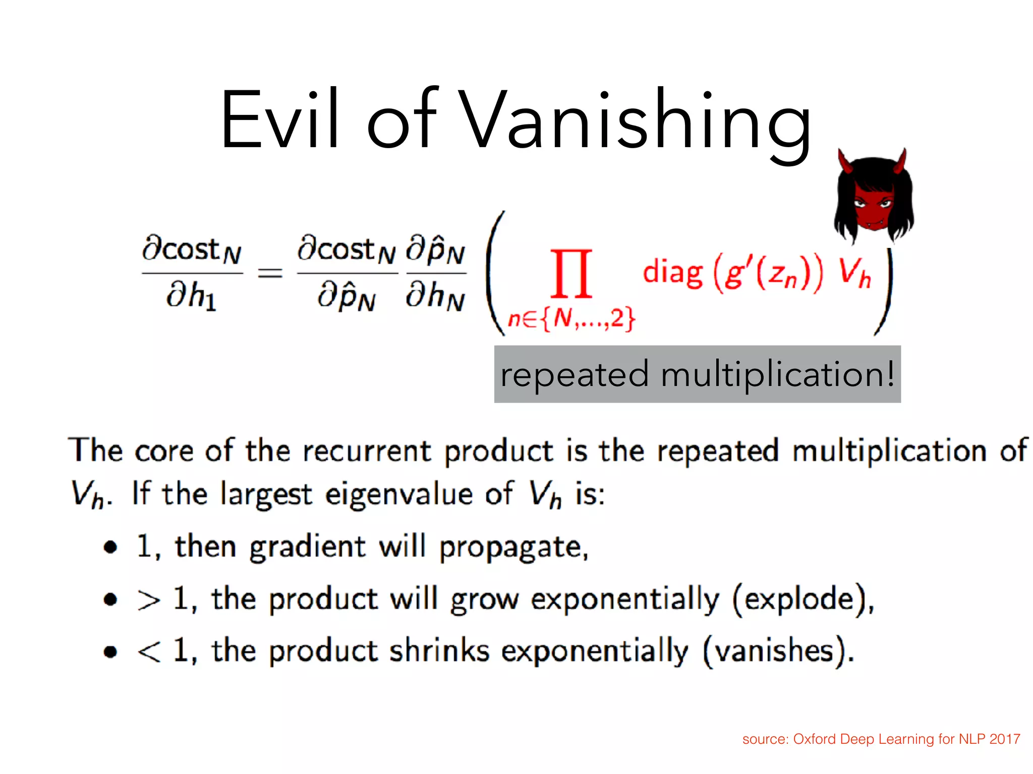
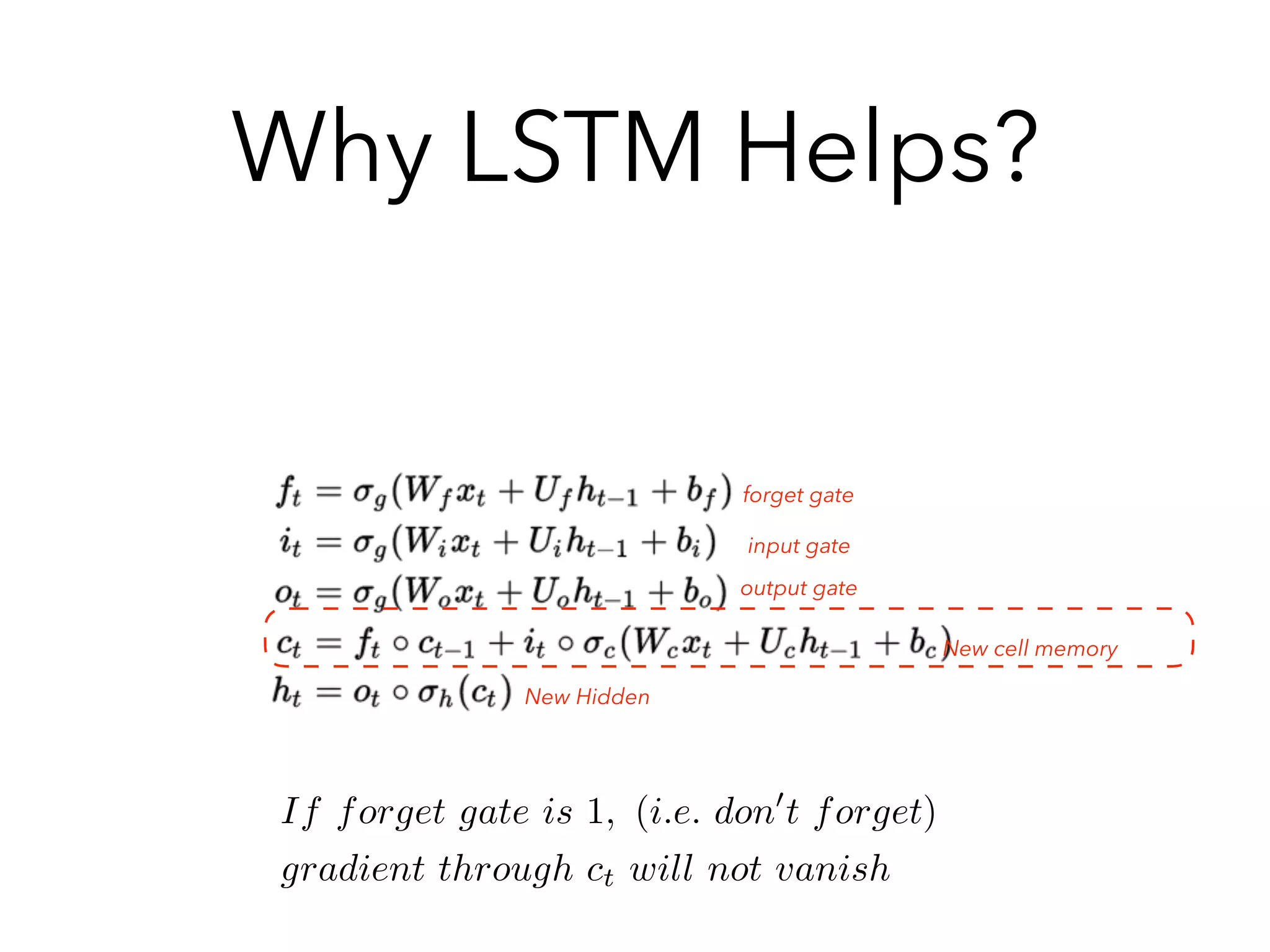
46. Why Vanishing?
CS 224d Richard Soucher
Jacobian Matrix
@Lt
@W
=
tX
k=1
@Lt
@ˆyt
@ˆyt
@ht
@ht
@hk
@hk
@W
@ht
@hk
= ⇧t
j=k+1
@hj
@hj 1
from step k to step t
@L
@W
=
tX
k=1
@Lt
@W
note :
@ht+1
i
@at+1
k
= 0, if k 6= iJacobian [
@ht+1
i
@ht
j
] =
X
k
@ht+1
i
@at+1
k
·
@at+1
k
@ht
j
=
@ht+1
i
@at+1
i
Wij
= (1 tanh2
(at+1
i ))Wij = diag(1 tanh2
(at+1
))W
= diag(1 (ht+1
)2
)W

47. @ht
@hk
= ⇧t
j=k+1
@hj
@hj 1
= ⇧t
j=k+1(diag[f0
(aj
)]W)
k
@hj
@hj 1
k  kdiag[f0
(aj)]kkWT
k  h W
k
@ht
@hk
k = k⇧t
j=k+1
@hj
@hj 1
k  ( h W )t k
CS 224d Richard Soucher
eg: t=200, k=5, both beta =0.9,
then almost 0
when both equals to 1.1,
17 digits.
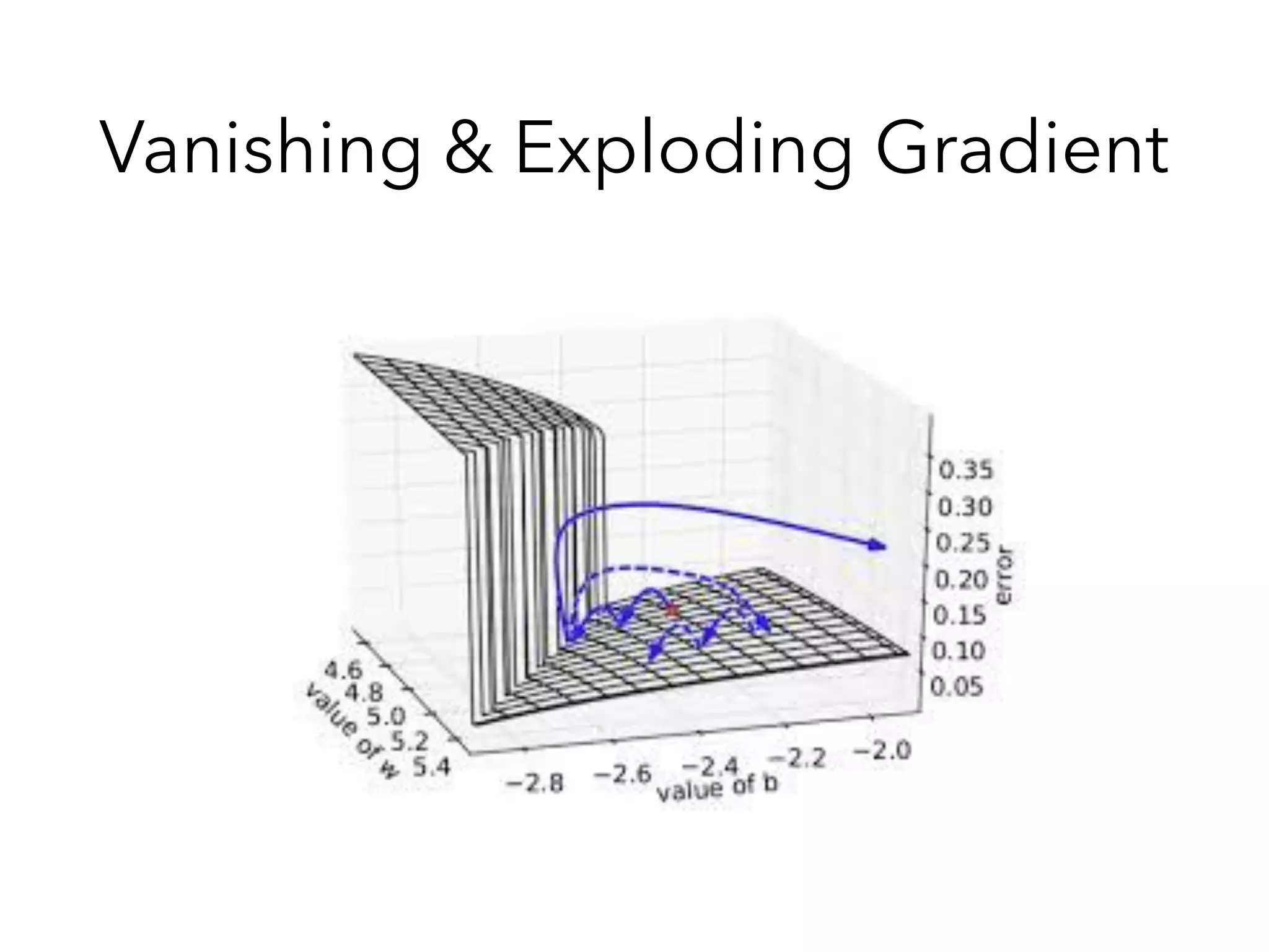
The Gradient Could be Exploded or Vanished!!!
Note: Vanishing/Exploding Gradient Not only happens in RNN, but also in Deep Feed Forward Network !
Why Vanishing?

48. Possible Solution
• Echo Statte Network
• Design Input weights and recurrent weight, so as max Eigen value nears 1
• Leaky units @ multiple time scale (fine-grained time and coarse time)
• Adding Skip Connection through time (every time d time steps)
• Leaky Units: Linear self-connected
• Removing Connection
• LSTM
• Regularizer to encourage info flow
µt
↵µt+1
+ (1 ↵)vt

49. Practical Measure
• Exploding Gradients
• Truncated BPTT (how many steps to BP)
• Clip Gradient at Threshold
• RMSProp to adjust learning rate
• Vanishing Gradient (harder to detect)
• Weight Initialization (Identity Matrix for W + Relu as Activation)
• RMSProp
• LSTM, GRU
Nervana Recurrent Neural Network
https://www.youtube.com/watch?v=Ukgii7Yd_cU

50. Using Gate & Extra Memory
LSTM, (GRU, Peephole)
Long Shot term Memory

51. Introducing Gate
•a vector
•1 or 0
•if 1, info will be kept
•if 0, info will be flushed
•Operation: Elementwise
dot
•Sigmoid is an intuitive
selection
•To be learned by NN
2
6
6
6
6
6
6
4
a1
a2
a3
aj
an
.
3
7
7
7
7
7
7
5
2
6
6
6
6
6
6
4
1
0
1
0
0
.
3
7
7
7
7
7
7
5
=
2
6
6
6
6
6
6
4
a1
0
a3
0
0
.
3
7
7
7
7
7
7
5
before aftergate

52. LSTM
Ct−1
ht−1
input gate
forget gate
output gate
New cell memory
New Hidden
colah.github.io

53. • Add Cell Memory C_t (so, 3 input, X_t, H_t, C_t)
• More Weigh Matrices to form Gate
• V. RNN Update Memory @ Every time step,
• LSTM update memory or not governed by Gate
LSTM vs Vanilla RNN

54. LSTM - Conveyer line
Carry or Flush
A conveyer line which could add/
remove ‘things’ from C(t-1) to C(t)
ft ⊙ Ct−1
ft ⊙ Ct−1 : ft applies to every element of Ct−1
to decide whether to carry/flush the info
colah.github.io
whether to forget

55. LSTM - info to Add/update
˜Ct : New info
it : input gate, similar to ft
so, it ⊙ ˜Ct : the info to be updated
Ct : Final contents in cell memory
colah.github.io

56. LSTM-what to output
ot : output gate, similar to it, ft
To get target output ht : First, Ct into tanh (to ensure between − 1, 1), then dot product with ot
colah.github.io

57. LSTM- Whole Picture
Ct−1
ht−1
ht
Ct
Forget Gate Input Gate + New Info
Output Gate
colah.github.io

58. Why LSTM Helps on
Gradient Vanishing ?

59. Evil of Vanishing
source: Oxford Deep Learning for NLP 2017
repeated multiplication!

60. Why LSTM Helps?
source: Oxford Deep Learning for NLP 2017
Adopt Additional memory cell,
RNN ‘LSTM’
f i
from ⇤ to +

61. source: Oxford Deep Learning for NLP 2017
if forget gate is equal 1, then gradient could trace all back to the original
Why LSTM Helps?

62. input gate
forget gate
output gate
New cell memory
New Hidden
If forget gate is 1, (i.e. don0
t forget)
gradient through ct will not vanish
Why LSTM Helps?

63. Why LSTM Could help Gradient
Passing
• The darker the shade, the greater the sensitivity
• The sensitivity decays exponentially over time as new inputs overwrite the
activation of hidden unit and the network ‘forgets’ the first input
• Traditional RNN updates hidden state in Every Step, while, LSTM using extra
‘memory’ to keep and update till needed
• Memory cells are additive in time
Loss

64. Graph in the BookCHAPTER 10. SEQUENCE MODELING: RECURRENT AND RECURSIVE NETS
at each time step.
×
input input gate forget gate output gate
output
state
self-loop
×
+ ×
Figure 10.16: Block diagram of the LSTM recurrent network “cell.” Cells are connected
recurrently to each other, replacing the usual hidden units of ordinary recurrent networks.
An input feature is computed with a regular artificial neuron unit. Its value can be
accumulated into the state if the sigmoidal input gate allows it. The state unit has a
linear self-loop whose weight is controlled by the forget gate. The output of the cell can

65. Notation in the book
f
(t)
i = σ(bf
i +
j
Uf
i,jx
(t)
j +
j
Wf
i,jh
(t−1)
j )
time step t and ith cell
g
(t)
i = σ(bg
i +
j
Ug
i,jx
(t)
j +
j
Wg
i,jh
(t−1)
j )
q
(t)
i = σ(bq
i +
j
Uq
i,jx
(t)
j +
j
Wq
i,jh
(t−1)
j )
outputgate
s
(t)
i = f
(t)
i s
(t−1)
i + g
(t)
i σ(bi +
j
Ui,jx
(t)
j +
j
Wi,jh
(t−1)
j )
forget gate
input gate
Memory Cell
h
(t)
i = tanh(s
(t)
t )qi(t)
Final output/hidden
input gate
————————-New info———————————

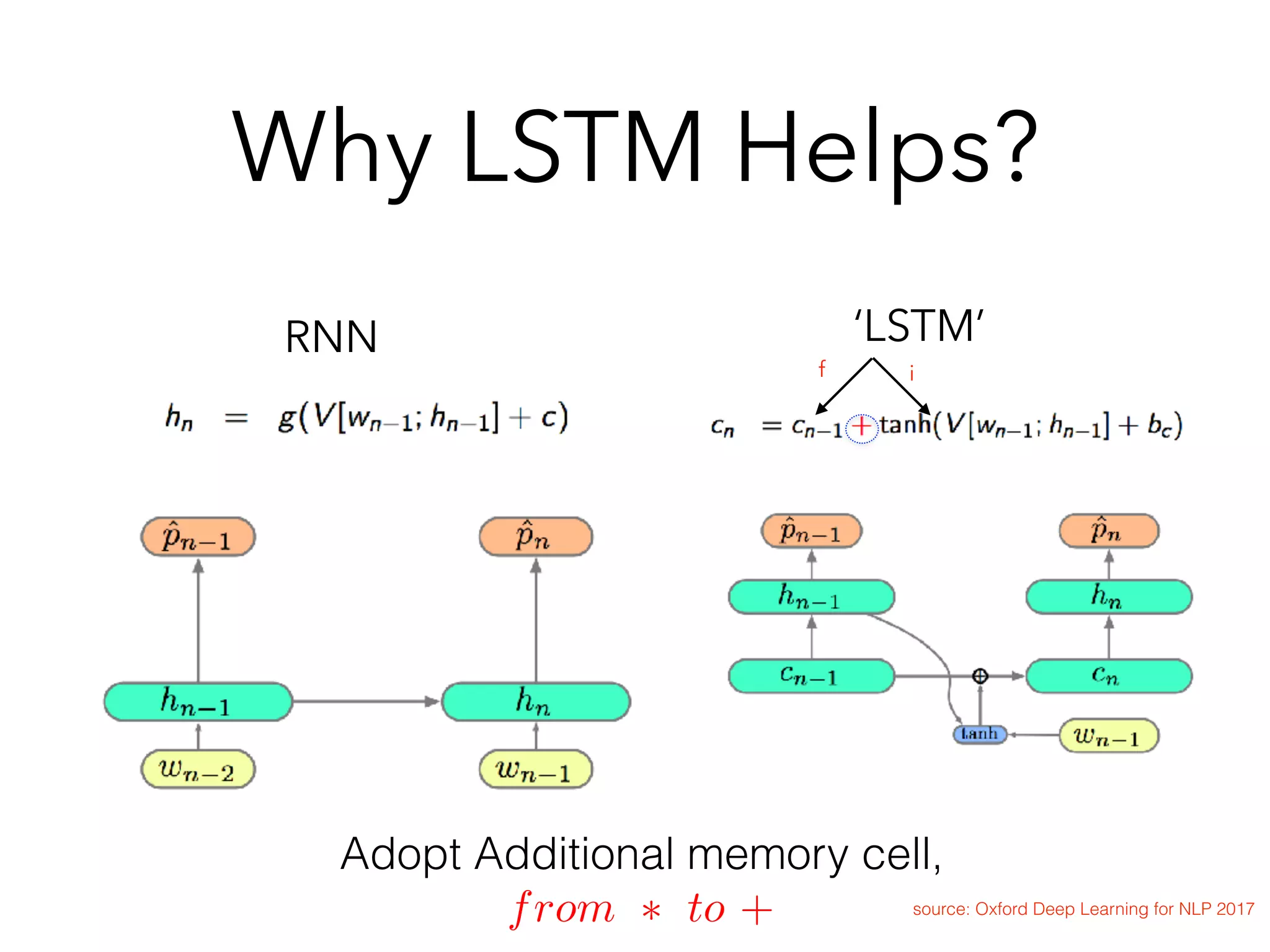
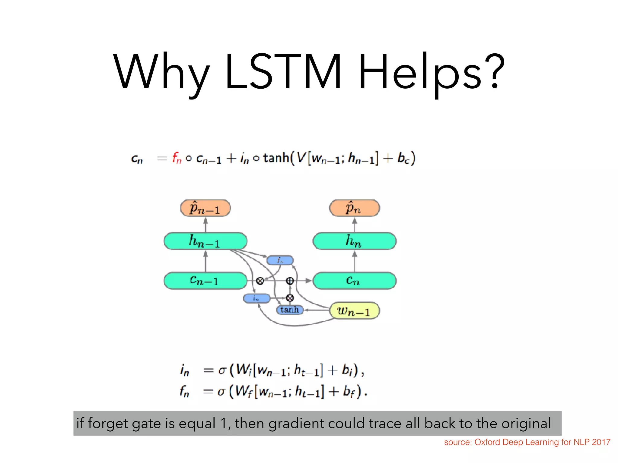
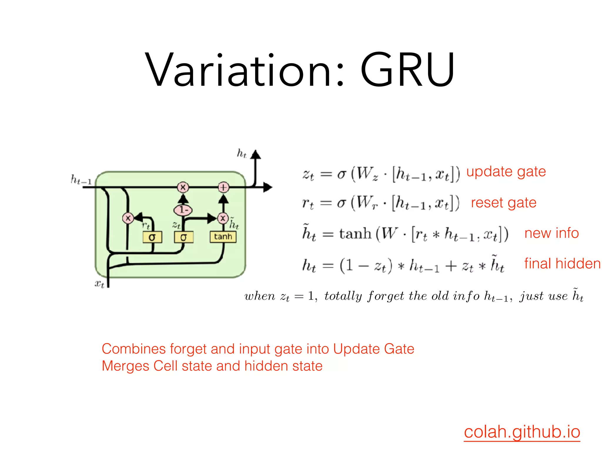
66. Variation : GRU
(Parameter reduction)
ht
= (1 zt
) • ht 1
+ zt
• ˜ht
LSTM is good but seems redundant?
Do we need so many gates ?
Do we need Hidden State AND Cell Memory to remember ?
zt
is a gate
˜ht
= tanh(Wxt
+ Uht 1
+ b)
vs.
˜ht
= tanh(Wxt
+ U(rt
• ht 1
) + b) rt
is a gate
More previous state info or More new Info ? Z^t will decide
zt
= (Wz[xt
; ht 1
] + bz) rt
= (Wr[xt
; ht 1
] + br)
can’t forget

67. Variation: GRU
Combines forget and input gate into Update Gate
Merges Cell state and hidden state
colah.github.io
update gate
reset gate
when zt = 1, totally forget the old info ht 1, just use ˜ht
new info
final hidden

68. Variation： Peephole
colah.github.io
peephole: also consider C(t-1)
add Ct 1 as input

69. Comparison of Various LSTM
Models
1. Vanilla (V) (Peephole LSTM)
2. No Input Gate (NIG)
3. No Forget Gate (NFG)
4. No Output Gate (NOG)
5. No Input Activation Function (NIAF)
6. No Output Activation Function (NOAF)
7. No Peepholes (NP)
8. Coupled Input and Forget Gate (CIFG, GRU)
9. Full Gate Recurrence (FGR, adding All gate recurrence)
1. TIMIT Speech corpus (Garofolo et
al., 1993)
2. IAM Online Handwriting Database
(Liwicki & Bunke, 2005)
3. JSB Chorales (Allan & Williams,
2005)
Source: LSTM: A Search Space Odyssey

70. Result, Just V or GRU
Overall, Vanilla and GRU have the best
result!!
in tensorflow,
BasicLSTM doesn’t include Peephole
LSTMcell have the option:
use_peepholes=False

71. Advise on Training (gated) RNN
• Use an LSTM or GRU: it makes your life so much simpler!
• Initialize recurrent matrices to be orthogonal
• Initialize other matrices with a sensible (small!) scale
• Initialize forget gate bias to 1: default to remembering
• Use adaptive learning rate algorithms: Adam, AdaDelta, ...
• Clip the norm of the gradient: 1–5 seems to be a reasonable
threshold when used together with Adam or AdaDelta.
• Either only dropout vertically or learn how to do it right
• Be patient! source: Oxford Deep Learning for NLP 2017
[Saxe et al., ICLR2014;
Ba, Kingma, ICLR2015;
Zeiler, arXiv2012;

72. Real World Application

73. Image Captioning
Source: Andrej Karpathy, Fei-Fei Li cs231n

74. Image Captioning
Source: Andrej Karpathy, Fei-Fei Li cs231n

75. Image Captioning
Source: Andrej Karpathy, Fei-Fei Li cs231n
Transfer learning via
ImageNet
then RNN

76. SVHN: from CNN to
CNN+RNN

77. Case: SVHN(Multi Digit)
Street Video House Number in Real World

78. SVHN (Single Digit)
Colored MNIST ??!

79. It Works for SVHN

80. Data Preprocessing
10 classes, 1 for each digit. Digit '1' has label 1, '9' has label 9 and '0' has label
10.
73,257 digits for training, 26,032 digits for testing, and 531,131 additional
Comes in two formats:
Original images with character level bounding boxes.
MNIST-like 32-by-32 images centered around a single character
Significantly harder, unsolved, real world problem (recognizing digits and
numbers in natural scene images).
HDF5 format!!!! (what is this!!..)
n*Bounded Boxes Coordinate (for n digits)
Read in Data, Find Maximum Bounded Box and Crop.
Rotation (within +- 45 degree) and Scale
Color to Grayscale
Normalization
can't use extra dataset!
Memory overflow!!
Data: Google Street Video
Multi digit

81. Architect Labeling & Network
2
6
6
6
6
6
6
4
0
0
.
1
.
.
3
7
7
7
7
7
7
5
2
6
6
6
6
6
6
4
0
0
.
1
.
.
3
7
7
7
7
7
7
5
2
6
6
6
6
6
6
4
0
0
.
1
.
.
3
7
7
7
7
7
7
5
2
6
6
6
6
6
6
4
0
0
.
1
.
.
3
7
7
7
7
7
7
5
2
6
6
6
6
6
6
4
0
0
.
1
.
.
3
7
7
7
7
7
7
5
2
6
6
6
6
6
6
4
0
0
.
1
.
.
3
7
7
7
7
7
7
5
6 digit, first digit,
1st: number of digits,
1-5 House Addresses
11 classes, 0-9,
10 for empty
actually, 1st digit is redundant
CNN*3 with Pool
Drop out
Flattened
Fully Connected*6
Softmax & Cross Entropy
Network Architecture
digit 1
digit 2
digit 3
digit 4
digit 5
digit 6
W1
W1
W2
W3

82. CNN+RNN
Fully Connected Layer as input
SAME INPUT for different time steps!
One Layer LSTM
LSTM LSTM LSTM LSTM
LSTM
digit1 digit2 digit3 digit4 digit5
LSTM
digit0
x0 x1 x2 x3 x4 x5
O0 O1 O2 O3 O4 O5
Softmax

83. Result
Best: 69.7% Best: 76.5%
3 Layer CNN 3 Layer CNN+1 Layer RNN
• Note:
• This experiment is not ‘accurate’..
• Extend CNN to 5 layer, may help (around 72%…didn’t save..)
• Could be improved if adding LSTM drop out …etc.
• Should be Significantly Improved if Taking Extra (531K) dataset
• Tried Transfer Learning, apply inception v3…(有蟲..)....

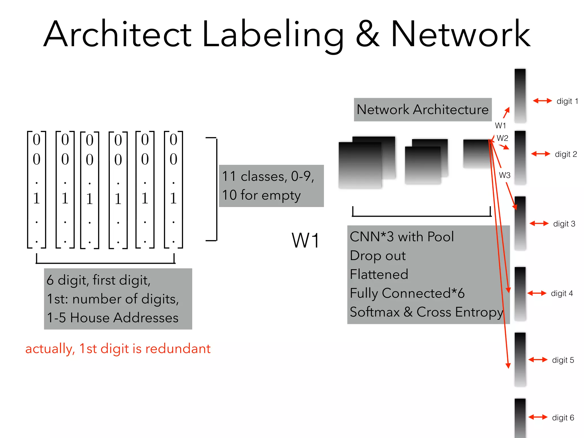
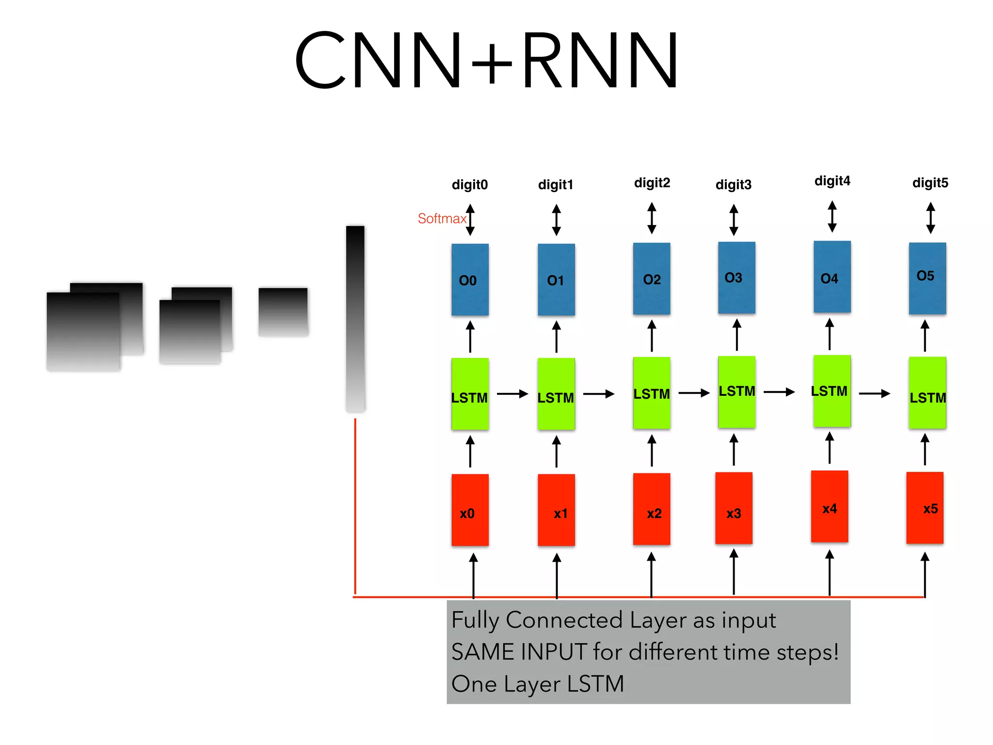
84. Some Experience(tensorflow)
• Input: [Batch, Time_steps, Input_length]
• If for a Image: Time_steps = Height, Input Length= Width
• Tf.unstack (input, 1) = list [[Batch, Input_length],[Batch,
Input_length], ……
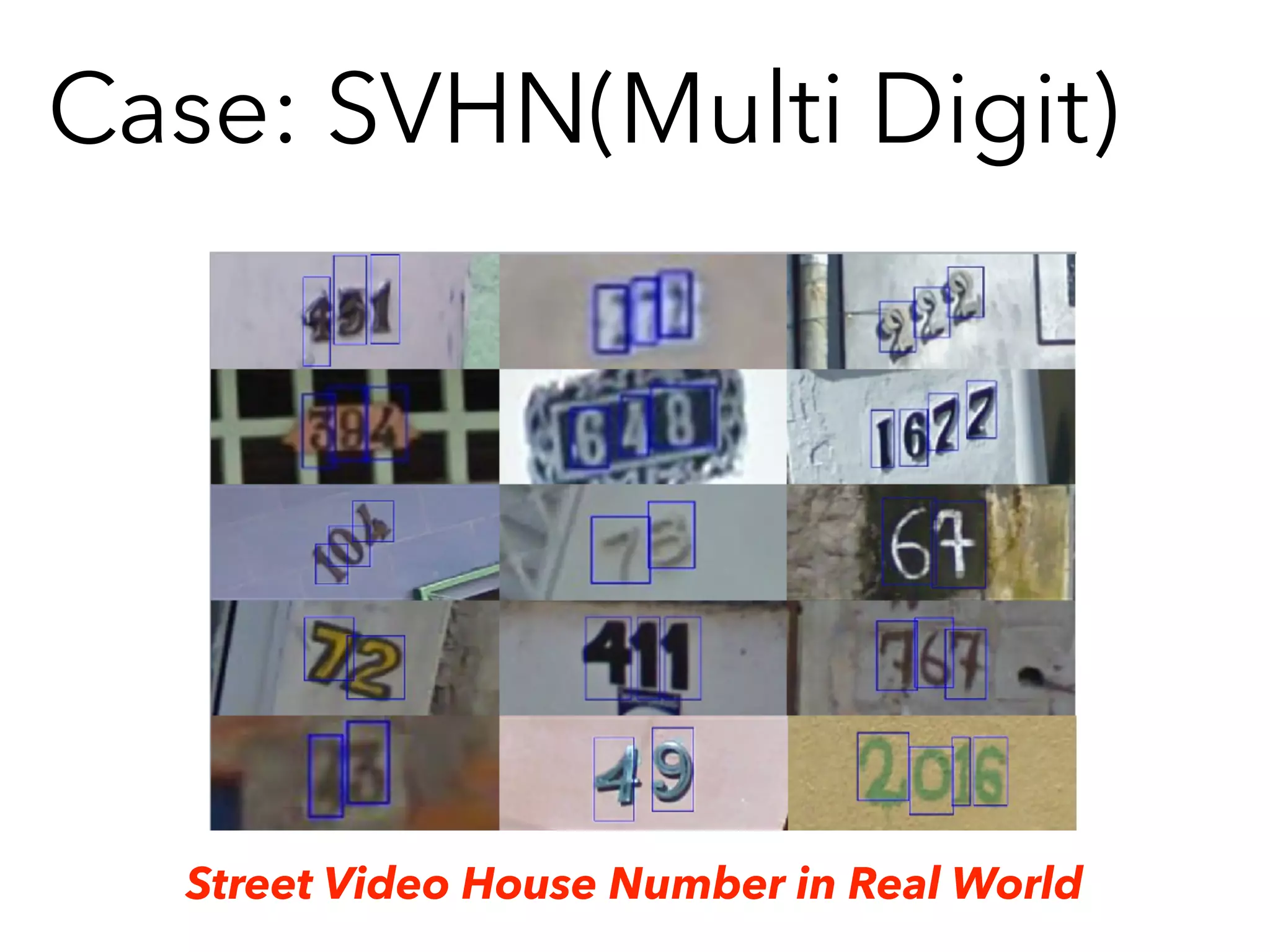
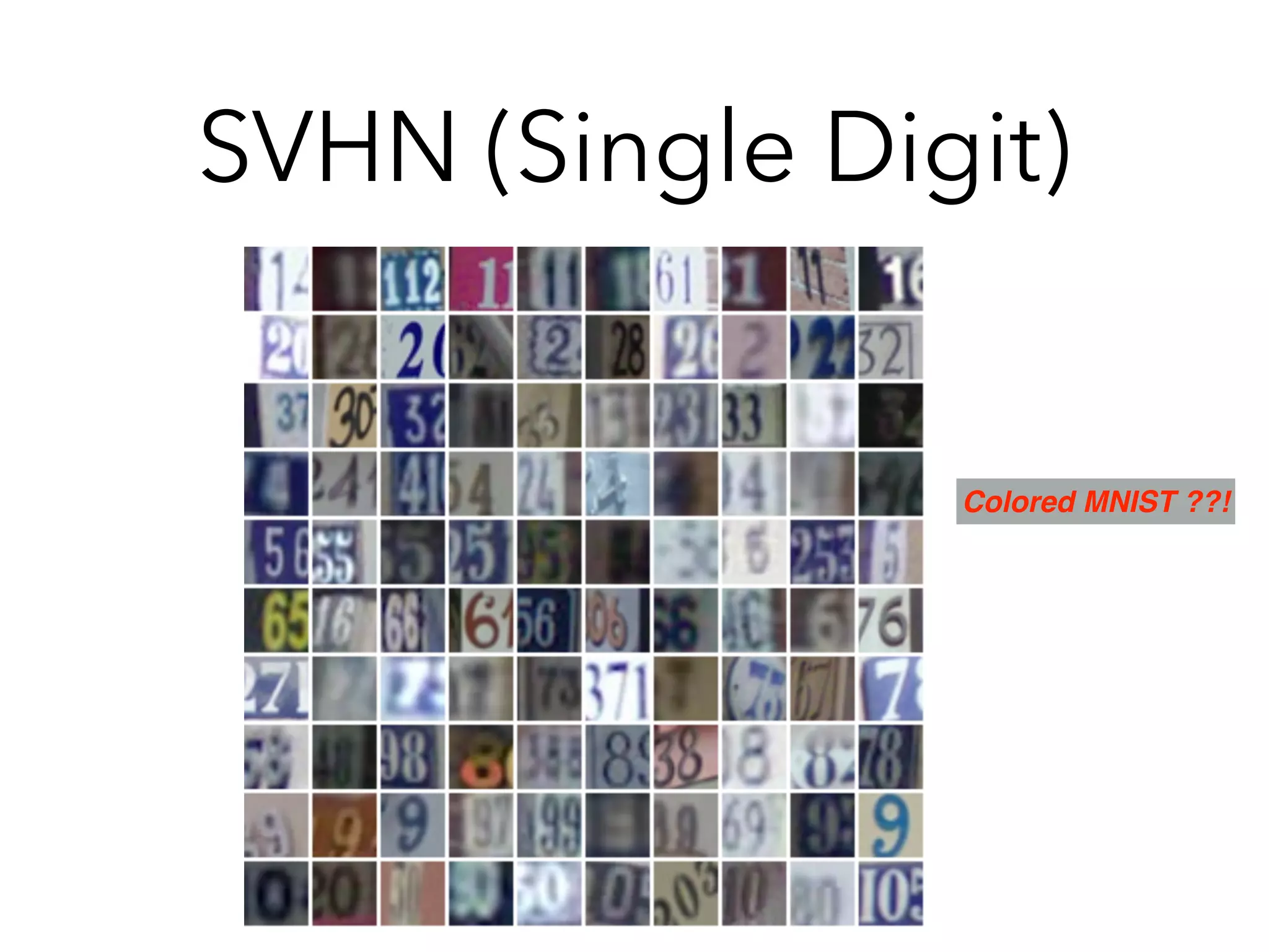
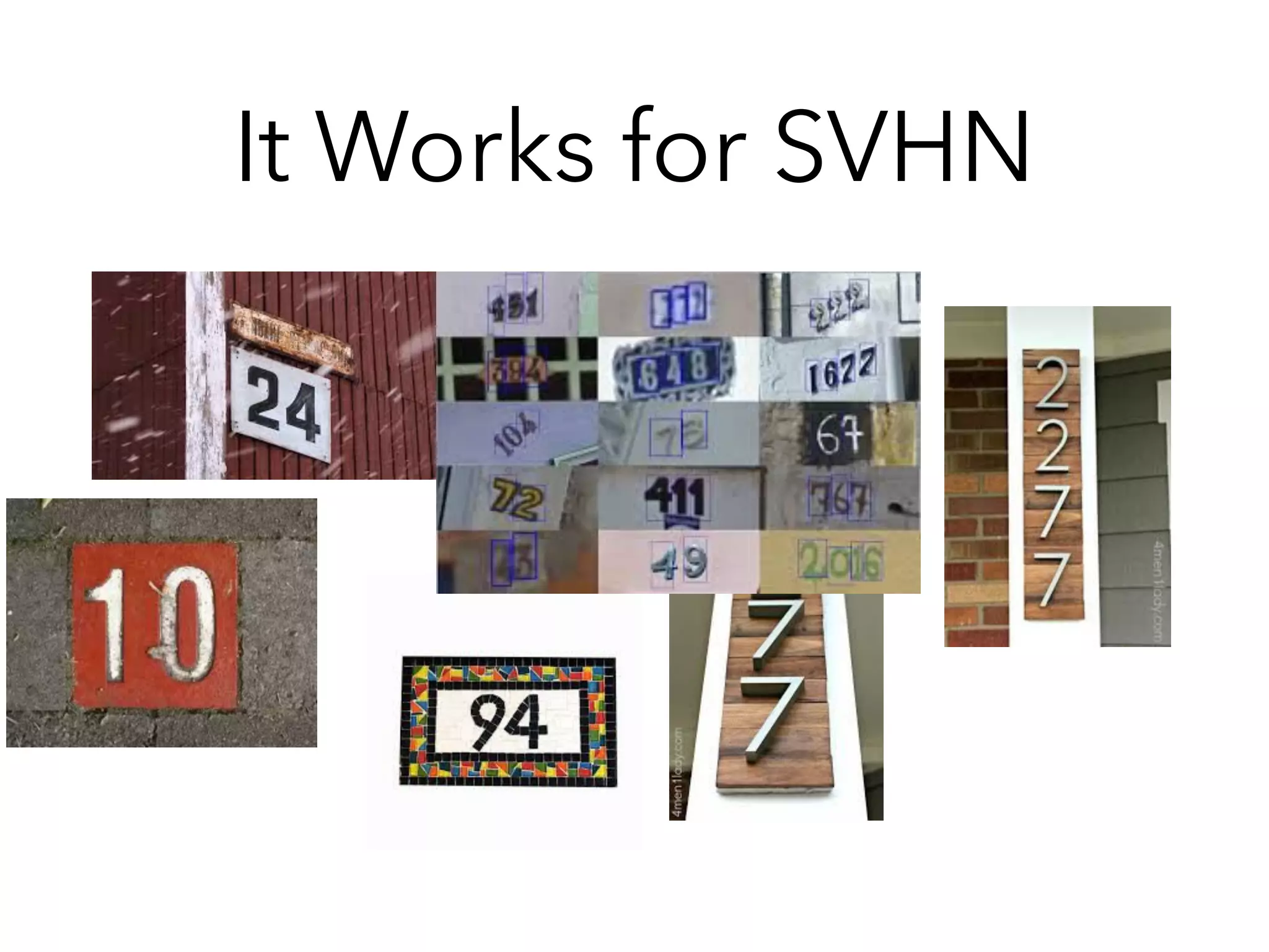
• Experience Using CNN+RNN for SVHN:
• Image - CNN - Flatten Feature Vectors (No go to Softmax)
• [Feature Vector, Feature Vector, Feature Vector…]as Inputs
Time_step1
Time_step2
a list of time step
Feature Vector*6

85. Chatbot &
Sequence to Sequence
By Ryan Chao
(ryanchao2012@gmail.com)

86. Language Model
Background knowledge
A statistical language model is a probability distribution over sequences of words. (wiki)
n-gram model

87. Background knowledge
n-gram model
bigram(n = 2)
trigram(n = 3)
Language Model
A statistical language model is a probability distribution over sequences of words. (wiki)

88. Background knowledge
Continuous Space Language Models - word embedding
Word2Vec NLM
Yoshua Bengio, Réjean Ducharme, Pascal Vincent, and Christian Janvin. 2003. A neural probabilistic language model. J. Mach. Learn. Res. 3 (March 2003), 1137-1155.

89. Cho, K., van Merriënboer, B., Gulcehre, C., Bougares, F., Schwenk, H., and Bengio, Y. (2014a).
Learning phrase representations using RNN encoder-decoder for statistical machine translation.
Novel Approach for Machine Translation
RNN Encoder–Decoder (with GRU)
GRU
Reset gate
Update gate
Background knowledge

90. Sequence to Sequence Framework by Google
1. Deeper Architecture: 4 layers
2. LSTM Units
3. Input Sentences Reversing
arXiv:1409.3215 (2014)
For solving “minimal time lag”:
“Because doing so introduces many short term dependencies
in the data that make the optimization problem much easier.”
I love you
you love I
Ich liebe dich <eos>
Background knowledge

91. Sequence to Sequence Framework by Google
1. Deeper Architecture: 4 layers
image source: http://suriyadeepan.github.io/2016-12-31-practical-seq2seq/
arXiv:1506.05869 (2015)
IT Helpdesk
Movie Subtitles
2. LSTM Units
3. Input Sentences Reversing
Background knowledge

92. Sequence to Sequence Framework by Google
arXiv:1409.3215, arXiv:1506.05869
Details of hyper-parameters: Total parameters to be trained:
Depth(each): 4 layers
Hidden Units in each layer: 1000 cells
Dimensions of word embedded: 1000
Input Vocabulary Size: 160,000 words
Output Vocabulary Size: 80,000 words
384 M
1k cell LSTM
1k cell LSTM
1k cell LSTM
1k cell LSTM
1k cell LSTM
1k cell LSTM
1k cell LSTM
1k cell LSTM
embedding lookup (160k) embedding lookup (80k)
softmax (80k)hidden vector (context)
Background knowledge

93. Sequence to Sequence Framework by Google
arXiv:1409.3215, arXiv:1506.05869
Depth(each): 4 layers
Hidden Units in each layer: 1000 cells
Dimensions of word embedded: 1000
Input Vocabulary Size: 160,000 words
Output Vocabulary Size: 80,000 words
Details of hyper-parameters: Total parameters to be trained:
384 M
1k cell LSTM
1k cell LSTM
1k cell LSTM
1k cell LSTM
1k cell LSTM
1k cell LSTM
1k cell LSTM
1k cell LSTM
embedding lookup (160k) embedding lookup (80k)
softmax (80k)hidden vector (context)
4 x 1k x 1k x 8 = 32 M = 32 M
Background knowledge

94. Sequence to Sequence Framework by Google
arXiv:1409.3215, arXiv:1506.05869
Depth(each): 4 layers
Hidden Units in each layer: 1000 cells
Dimensions of word embedded: 1000
Input Vocabulary Size: 160,000 words
Output Vocabulary Size: 80,000 words
Details of hyper-parameters: Total parameters to be trained:
384 M
1k cell LSTM
1k cell LSTM
1k cell LSTM
1k cell LSTM
1k cell LSTM
1k cell LSTM
1k cell LSTM
1k cell LSTM
embedding lookup (160k) embedding lookup (80k)
softmax (80k)
160k x 1k = 160 M 80k x 1k = 80 M
80k x 1k = 80 Mhidden vector (context)
4 x 1k x 1k x 8 = 32 M = 32 M
Encoder: 160 M + 32 M = 192 M Decoder: 80 M + 32 M + 80 M = 192 M
Background knowledge

95. Chit-chat Bot Messenger interface

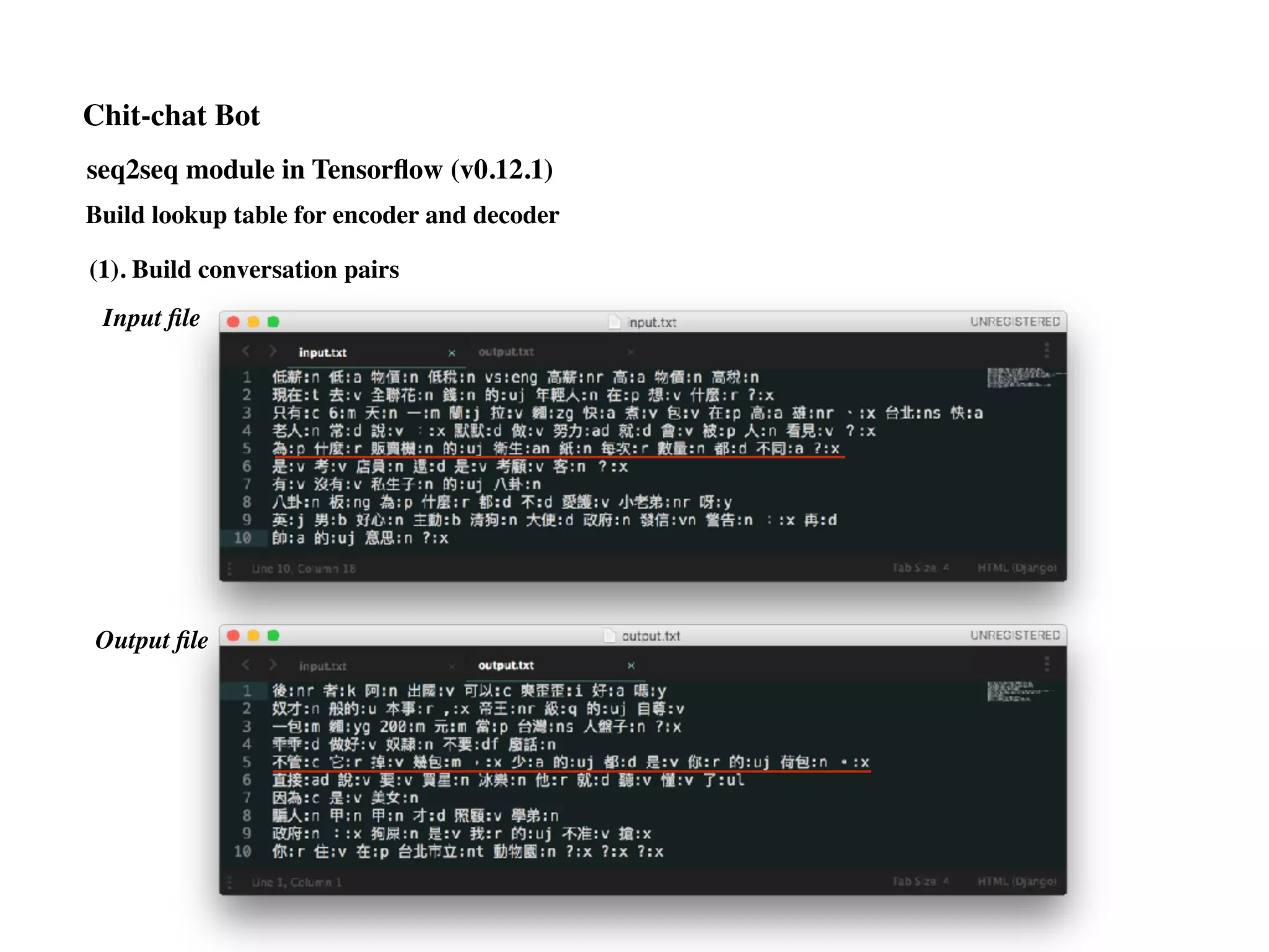
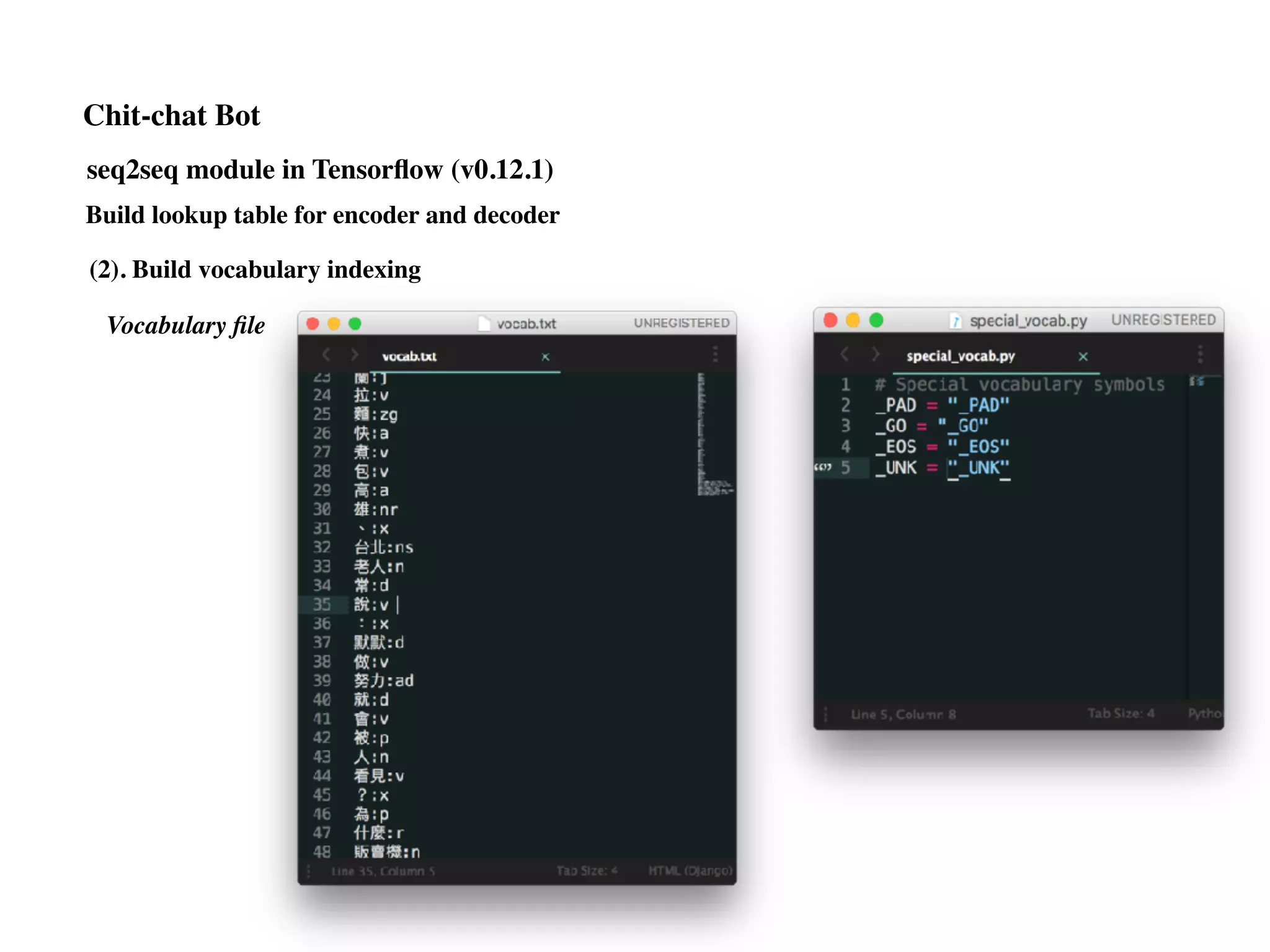
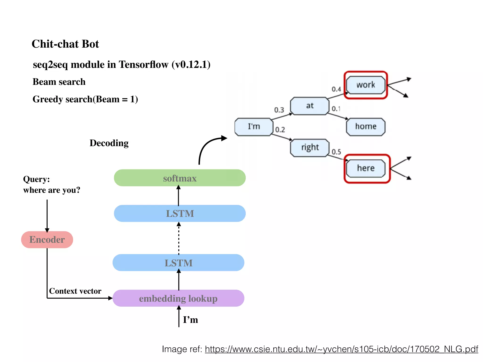
96. seq2seq module in Tensorflow (v0.12.1)
from tensorflow.models.rnn.translate import seq2seq_model
$> python translate.py
--data_dir [your_data_directory] --train_dir [checkpoints_directory]
--en_vocab_size=40000 --fr_vocab_size=40000
$> python translate.py --decode
--data_dir [your_data_directory] --train_dir [checkpoints_directory]
https://www.tensorflow.org/tutorials/seq2seq
Training
Decoding
Data source for demo in tensorflow:
WMT10(Workshop on statistical Machine Translation) http://www.statmt.org
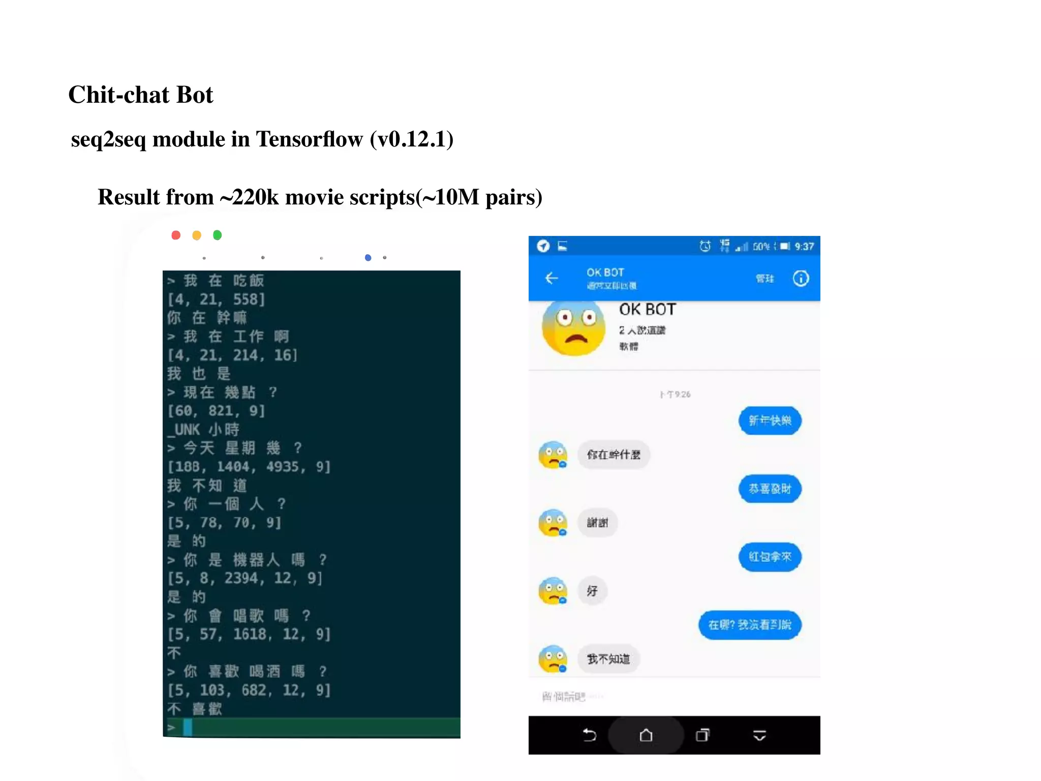
Data source for chit-chat bot:
Movie scripts, PTT corpus
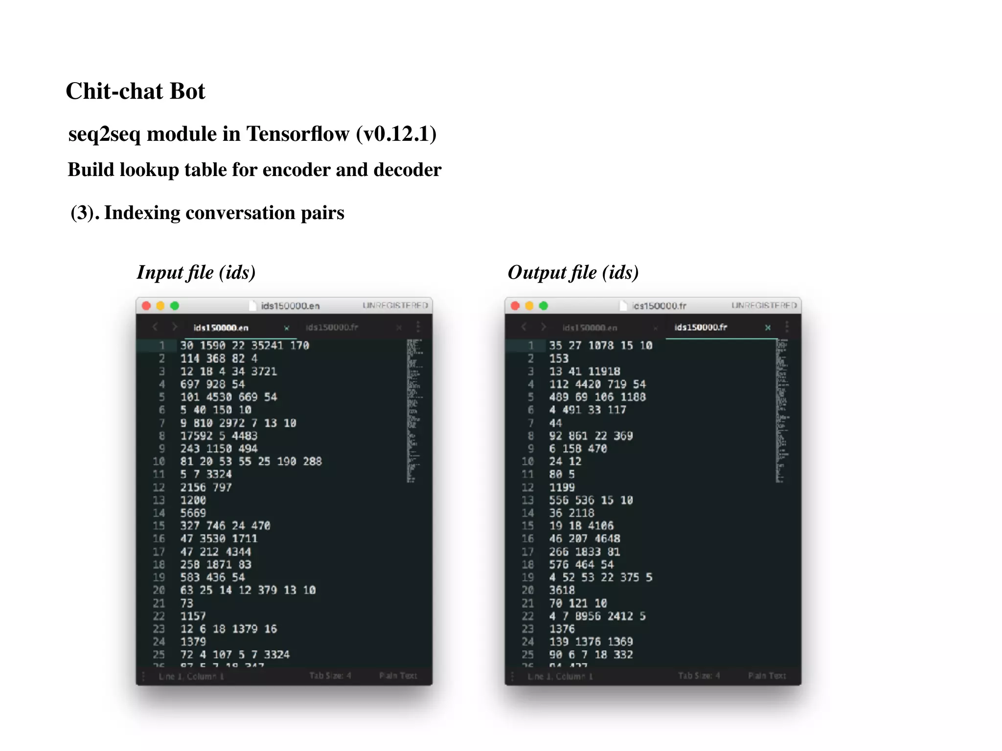
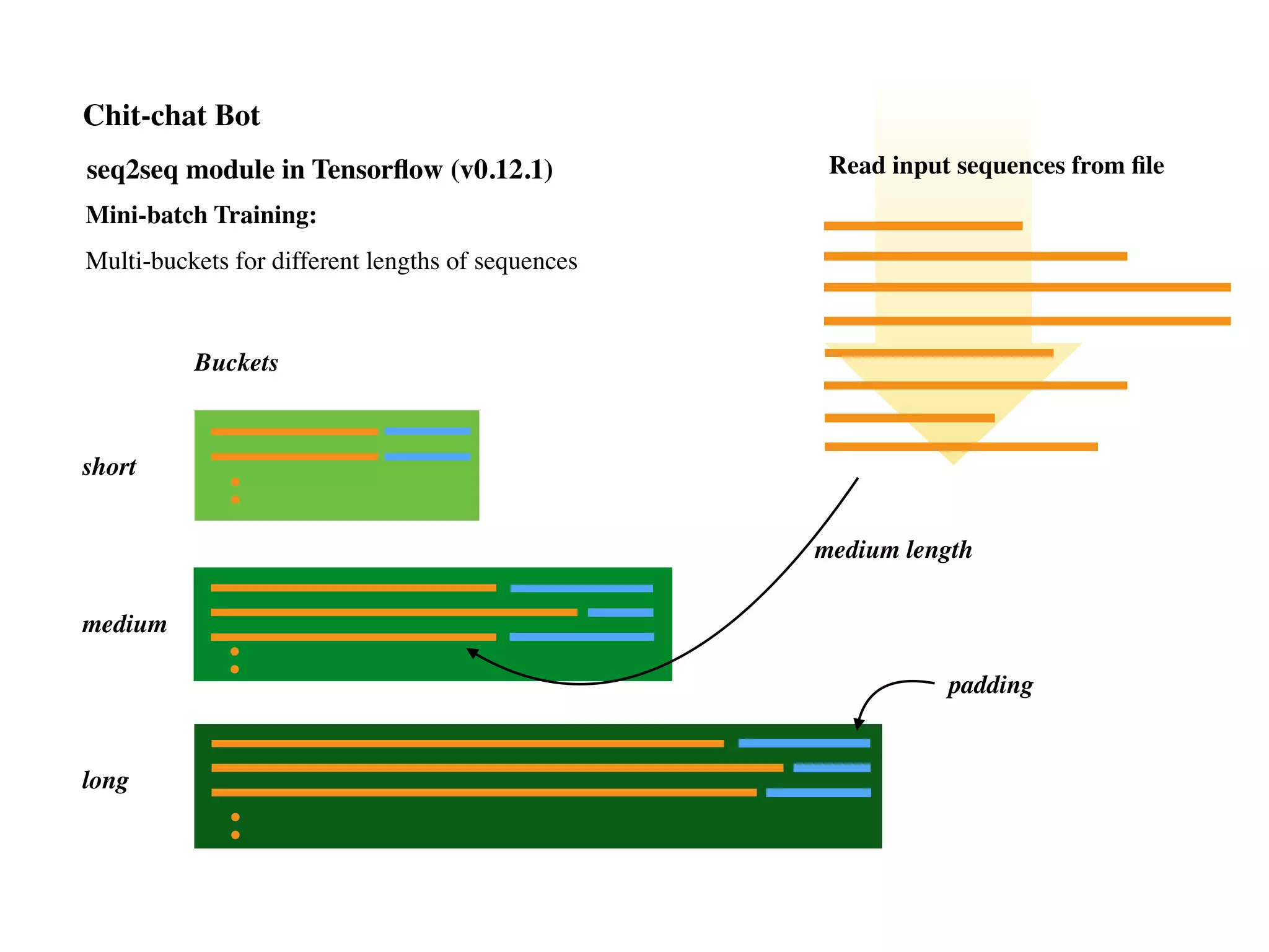
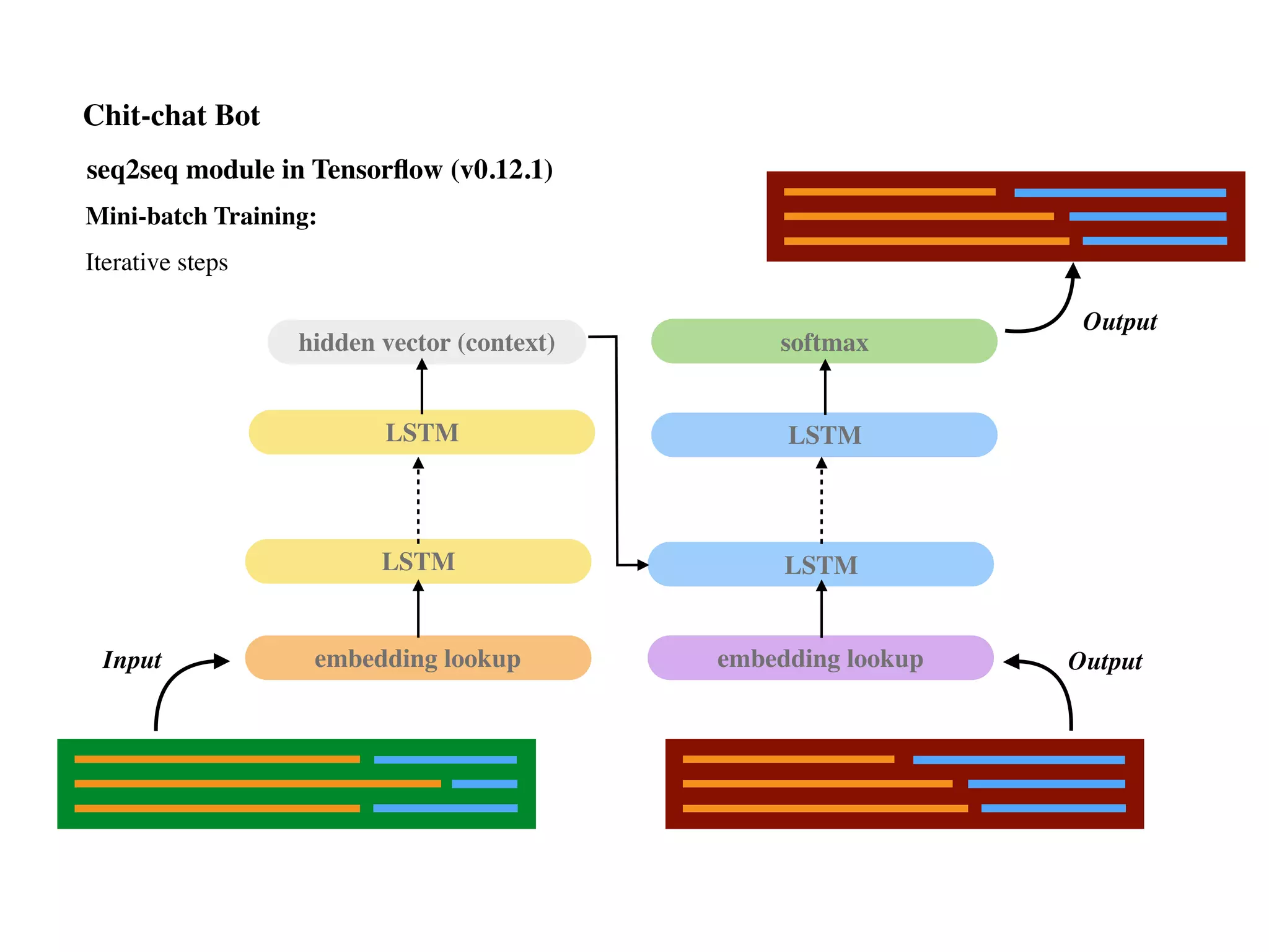
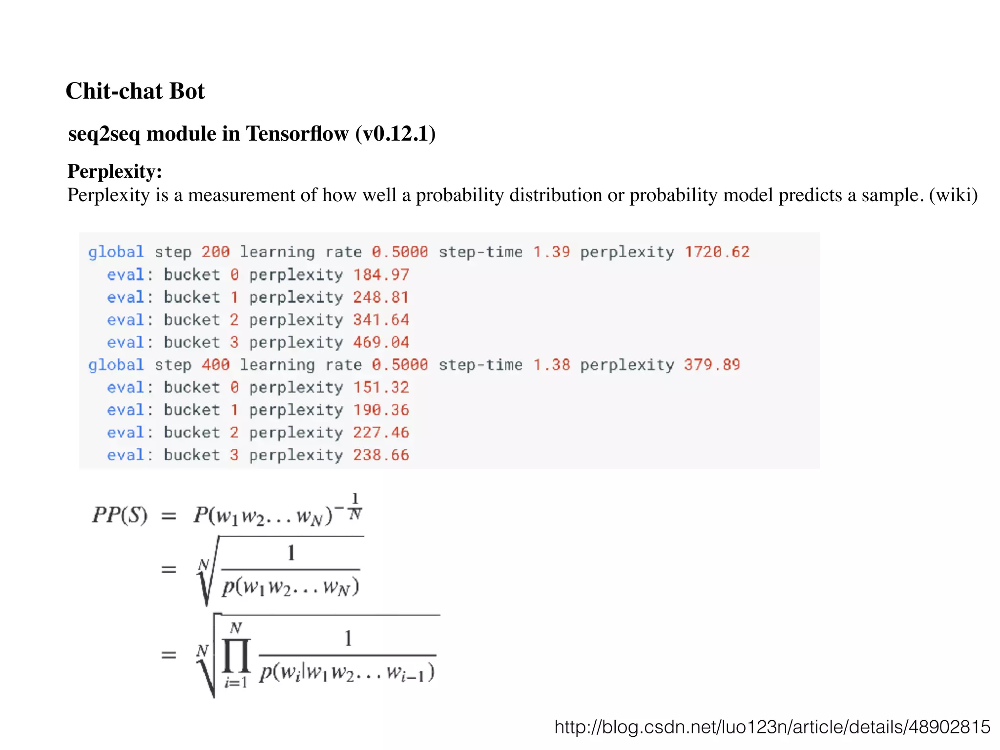
Chit-chat Bot
https://google.github.io/seq2seq/
new version

97. (1). Build conversation pairs
Input file
Output file
Build lookup table for encoder and decoder
Chit-chat Bot
seq2seq module in Tensorflow (v0.12.1)

98. (2). Build vocabulary indexing
Vocabulary file
Chit-chat Bot
Build lookup table for encoder and decoder
seq2seq module in Tensorflow (v0.12.1)

99. (3). Indexing conversation pairs
Input file (ids) Output file (ids)
Chit-chat Bot
Build lookup table for encoder and decoder
seq2seq module in Tensorflow (v0.12.1)

100. short
medium
long
Read input sequences from file
medium length
padding
Buckets
Chit-chat Bot
Mini-batch Training:
Multi-buckets for different lengths of sequences
seq2seq module in Tensorflow (v0.12.1)

101. LSTM
LSTM
LSTM
LSTM
embedding lookup embedding lookup
softmaxhidden vector (context)
Input
Output
Chit-chat Bot
Mini-batch Training:
Iterative steps
Output
seq2seq module in Tensorflow (v0.12.1)

102. Chit-chat Bot
Perplexity:
Perplexity is a measurement of how well a probability distribution or probability model predicts a sample. (wiki)
seq2seq module in Tensorflow (v0.12.1)
http://blog.csdn.net/luo123n/article/details/48902815

103. Chit-chat Bot
Beam search
Greedy search(Beam = 1)
seq2seq module in Tensorflow (v0.12.1)
Image ref: https://www.csie.ntu.edu.tw/~yvchen/s105-icb/doc/170502_NLG.pdf
LSTM
LSTM
embedding lookup
softmax
Decoding
Context vector
I’m
Encoder
Query:
where are you?

104. Chit-chat Bot
seq2seq module in Tensorflow (v0.12.1)
Result from ~220k movie scripts(~10M pairs)

105. Chit-chat Bot
Dual encoder arXiv:1506.08909v3
The Ubuntu Dialogue Corpus- A Large Dataset for Research in Unstructured Multi-Turn Dialogue Systems
Good pair:
C: 晚餐/要/吃/什什麼/？
R: 麥當勞
Bad pair:
C: 放假/要/去/哪裡/玩/呢/？
R: 公道/價/八/萬/⼀一
http://www.wildml.com/2016/07/deep-learning-for-chatbots-2-retrieval-based-model-tensorflow/

106. Chit-chat Bot
Summary

107. Chit-chat Bot
Summary
1. Dataset matters (movie scripts vs ptt corpus)

108. Chit-chat Bot
Summary
1. Dataset matters (movie scripts vs ptt corpus)
2. Retrieval-based > Generative-based

109. Chit-chat Bot
Summary
1. Dataset matters (movie scripts vs ptt corpus)
2. Retrieval-based > Generative-based
3. seq2seq framework is powerful but still impractical (English vs 中⽂)

110. Thank you.