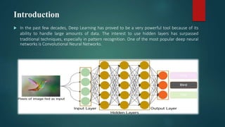
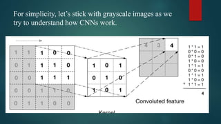
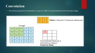
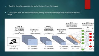
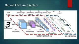
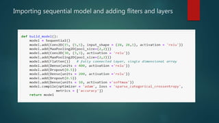
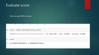
Convolutional neural networks (CNNs) are a type of deep neural network commonly used for analyzing visual imagery. CNNs use various techniques like convolution, ReLU activation, and pooling to extract features from images and reduce dimensionality while retaining important information. CNNs are trained end-to-end using backpropagation to update filter weights and minimize output error. Overall CNN architecture involves an input layer, multiple convolutional and pooling layers to extract features, fully connected layers to classify features, and an output layer. CNNs can be implemented using sequential models in Keras by adding layers, compiling with an optimizer and loss function, fitting on training data over epochs with validation monitoring, and evaluating performance on test data.

1. Convolutional
Neural Network

2. Introduction
 In the past few decades, Deep Learning has proved to be a very powerful tool because of its
ability to handle large amounts of data. The interest to use hidden layers has surpassed
traditional techniques, especially in pattern recognition. One of the most popular deep neural
networks is Convolutional Neural Networks.

3. APPLICATIONS
• OCR and image recognition
• Decoding Facial Recognition
• Analyzing Documents
• Grey Areas
• Detecting objects in self-driving cars
• Social media face recognition
• Image analysis in medicine
• Advertising

4. What exactly is a CNN?
 In deep learning, a convolutional neural network (CNN/ConvNet) is a class of deep neural networks, most
commonly applied to analyze visual imagery. Now when we think of a neural network we think about matrix
multiplications but that is not the case with ConvNet. It uses a special technique called Convolution. Now in
mathematics convolution is a mathematical operation on two functions that produces a third function that
expresses how the shape of one is modified by the other. But we don’t really need to go behind the mathematics part to
understand what a CNN is or how it works.
 Bottom line is that the role of the ConvNet is to reduce the images into a form that is easier to process, without losing features
that are critical for getting a good prediction.

5. Artificial Neural Network

7. Introduction
 Convolutional Neural Networks (CNNs) learns multi-level features and
 classifier in a joint fashion and performs much better than traditional
 approaches for various image classification and segmentation problems.

8. How does it work?
 Before we go to the working of CNN’s let’s cover the basics such as what is an image
and how is it represented. An RGB image is nothing but a matrix of pixel values
having three planes whereas a grayscale image is the same but it has a single plane.
Take a look at this image to understand more.

9. For simplicity, let’s stick with grayscale images as we
try to understand how CNNs work.

10. Convolution
• The primary purpose of Convolution in case of a CNN is to extract features from the input image.

11. Convolution...
 • The size of the output volume is controlled by three parameters that we need to decide
before the convolution step is performed:
 Depth: Depth corresponds to the number of filters we use for the convolution operation.
 Stride: Stride is the number of pixels by which we slide our filter matrix over the input
matrix.
 Zero-padding: Sometimes, it is convenient to pad the input matrix with zeros around the
border, so that we can apply the filter to bordering elements of our input image matrix.
• With zero-padding wide convolution
• Without zero-padding narrow convolution

12. Non-Linearity (ReLU)
 • Replaces all negative pixel values in the feature map by
zero.
 • The purpose of ReLU is to introduce nonlinearity in CNN,
since most of the real-worlddata would be non-linear.
 • Other non-linear functions such as tanh (-1,1) or sigmoid
(0,1) can also be used instead ofReLU (0,input).

13. Pooling
 Reduces the dimensionality of each feature map but retains the most important information.
Pooling can be of different types: Max, Average, Sum etc.

14.  • Together these layers extract the useful features from the images.
 • The output from the convolutional and pooling layers represent high-level features of the input
image.

15. Overall CNN Architecture

16. Putting it all together – Training using Backpropagation
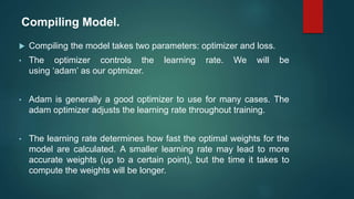
 • Step 1: We initialize all filters and parameters / weights with random values.
 • Step 2: The network takes a training image as input, goes through the forward propagation
step (convolution, ReLU and pooling operations along with forward propagation in the Fully
Connected layer) and finds the output probabilities for each class.
 • Let’s say the output probabilities for the boat image above are [0.2, 0.4, 0.1, 0.3].
 • Since weights are randomly assigned for the first training example, output probabilities are
also random.
 • Step 3: Calculate the total error at the output layer (summation over all 4 classes).

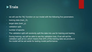
17.  Step 4: Use Backpropagation to calculate the gradients of the error with respect to all weights
in the network and use gradient descent to update all filter values/ weights and parameter
values to minimize the output error.
• The weights are adjusted in proportion to their contribution to the total error.
• When the same image is input again, output probabilities might now be [0.1, 0.1, 0.7, 0.1],
which is closer to the target vector [0, 0, 1, 0].
• This means that the network has learnt to classify this particular image correctly by adjusting its
weights / filters such that the output error is reduced.
• Parameters like number of filters, filter sizes, architecture of the network etc. have all been fixed
before Step 1 and do not change during training process – only the values of the filter matrix and
connection weights get updated.
 • Step 5: Repeat steps 2-4 with all images in the training set

18. • Parameters like number of filters, filter sizes, architecture of the network etc. have all
been fixed before Step 1 and do not change during training process – only the values of
the filter matrix and connection weights get updated.
 • Step 5: Repeat steps 2-4 with all images in the training set

19. SEQUENTIAL
 Model - Sequential
 Sequential is the easiest way to build a model in Keras. It allows you to build a model layer by
layer. Each layer has weights that correspond to the layer the follows it.
• We use the ‘add()’ function to add layers to our model.
• ‘Dense’ is the layer type. Dense is a standard layer type that works for most cases. In a dense layer, all
nodes in the previous layer connect to the nodes in the current layer.
 We define nodes in each of our input layers. This number can also be in the hundreds or
thousands. Increasing the number of nodes in each layer increases model capacity. I will go into
further detail about the effects of increasing model capacity shortly.
• ‘Activation’ is the activation function for the layer. An activation function allows models to take into
account nonlinear relationships.
 The first layer needs an input shape. The input shape specifies the number of rows and columns
in the input.
 The last layer is the output layer. It only has one node, two nodes as per requirment. which is for
our prediction.


20. Compiling Model.
 Compiling the model takes two parameters: optimizer and loss.
• The optimizer controls the learning rate. We will be
using ‘adam’ as our optmizer.
• Adam is generally a good optimizer to use for many cases. The
adam optimizer adjusts the learning rate throughout training.
• The learning rate determines how fast the optimal weights for the
model are calculated. A smaller learning rate may lead to more
accurate weights (up to a certain point), but the time it takes to
compute the weights will be longer.

21. Train
• we will use the ‘fit()’ function on our model with the following five parameters:
• training data (train_X),
• target data (train_y),
• validation split,
• number of epochs
• The validation split will randomly split the data into use for training and testing.
• During training, we will be able to see the validation loss, If we will set the
validation split at 0.2, which means that 20% of the training data we provide in
the model will be set aside for testing model performance.

22. • The number of epochs is the number of times the model will cycle through the
data. The more epochs we run, the more the model will improve, up to a certain
point. After that point, the model will stop improving during each epoch. In
addition, the more epochs, the longer the model will take to run. To monitor this,
we will use ‘early stopping’.
• Early stopping will stop the model from training before the number of epochs is
reached if the model stops improving. We will set our early stopping monitor to
3. This means that after 3 epochs in a row in which the model doesn’t improve,
training will stop. Sometimes, the validation loss can stop improving then
improve in the next epoch, but after 3 epochs in which the validation loss doesn’t
improve, it usually won’t improve again.
• to make predictions on new data, we would use the ‘predict()’ function, passing
in our new data.
 As you increase the number of nodes and layers in a model, the model capacity
increases. Increasing model capacity can lead to a more accurate model, up to
a certain point, at which the model will stop improving. Generally, the more
training data you provide, the larger the model should be.

23. Programming
importing libaries

24.  We import required libraries
 Importing Numpy , Pandas ,
 Importing Tensorflow As Tf
 From Tensorflow Import Keras
 Reading The Data

25. • Here we have 785 columns

26. Importing sequential model and adding fliters and layers

27. Running epochs

28. visualization

29. Evaluate score
• Here we got 98% accuracy

30. THANK YOU