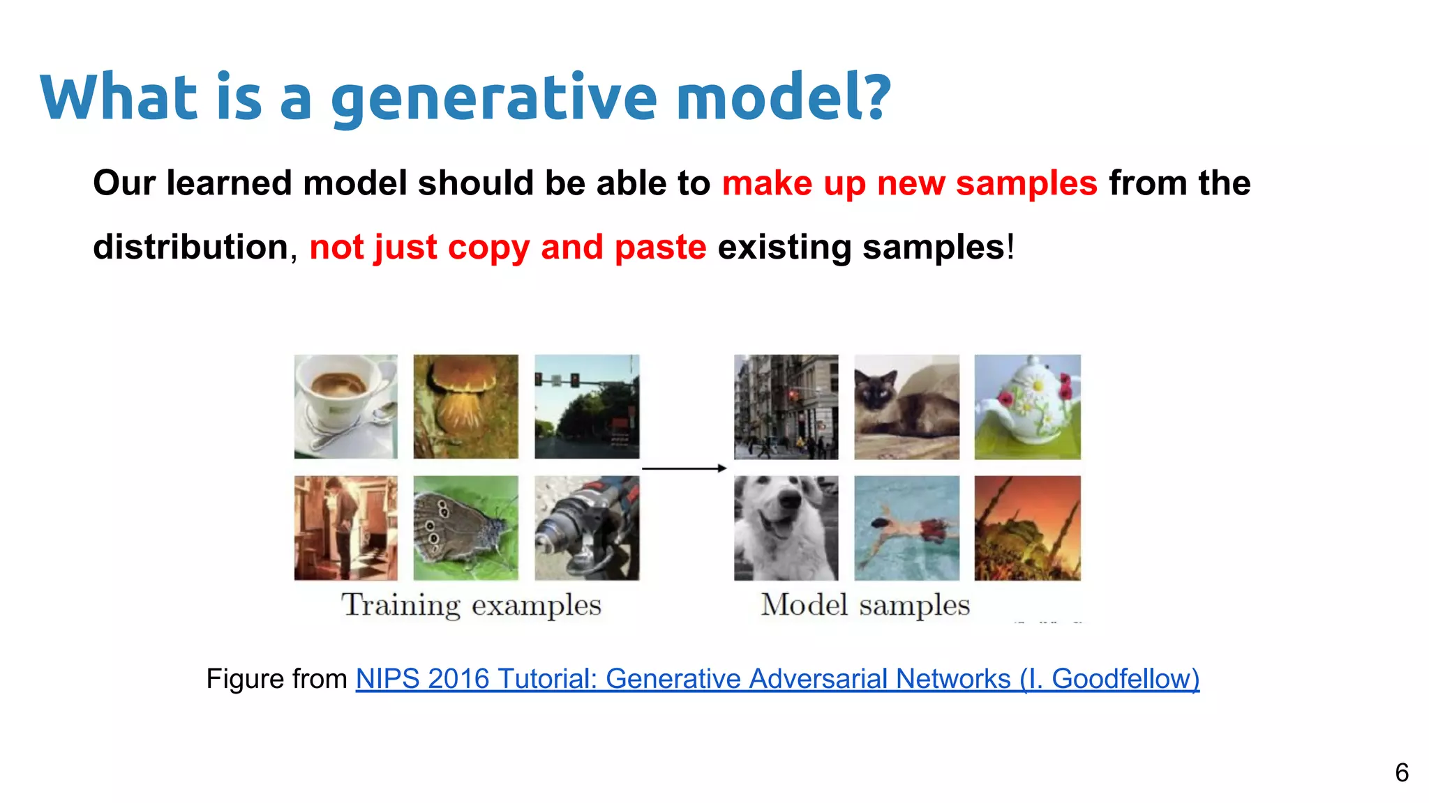
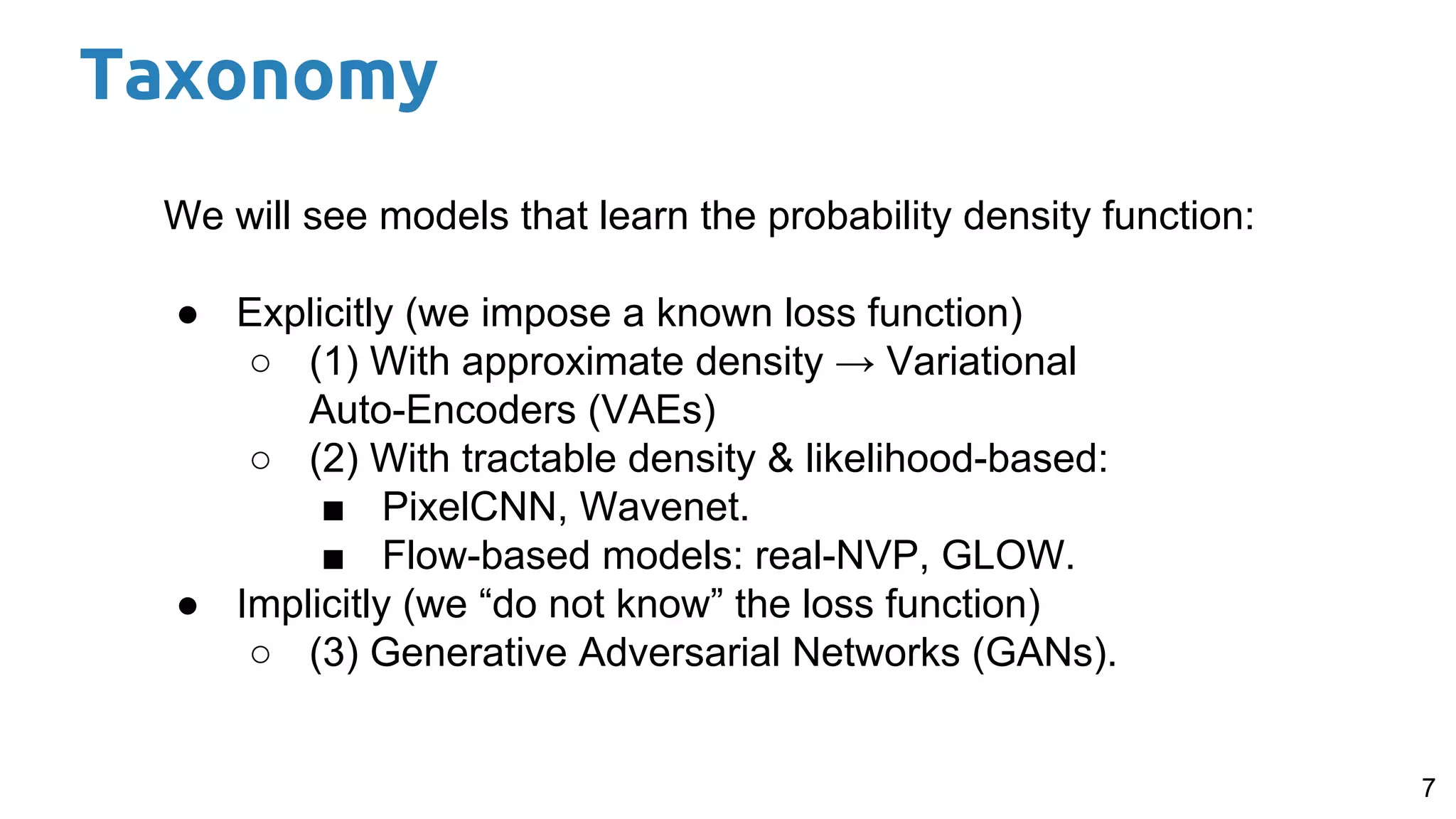
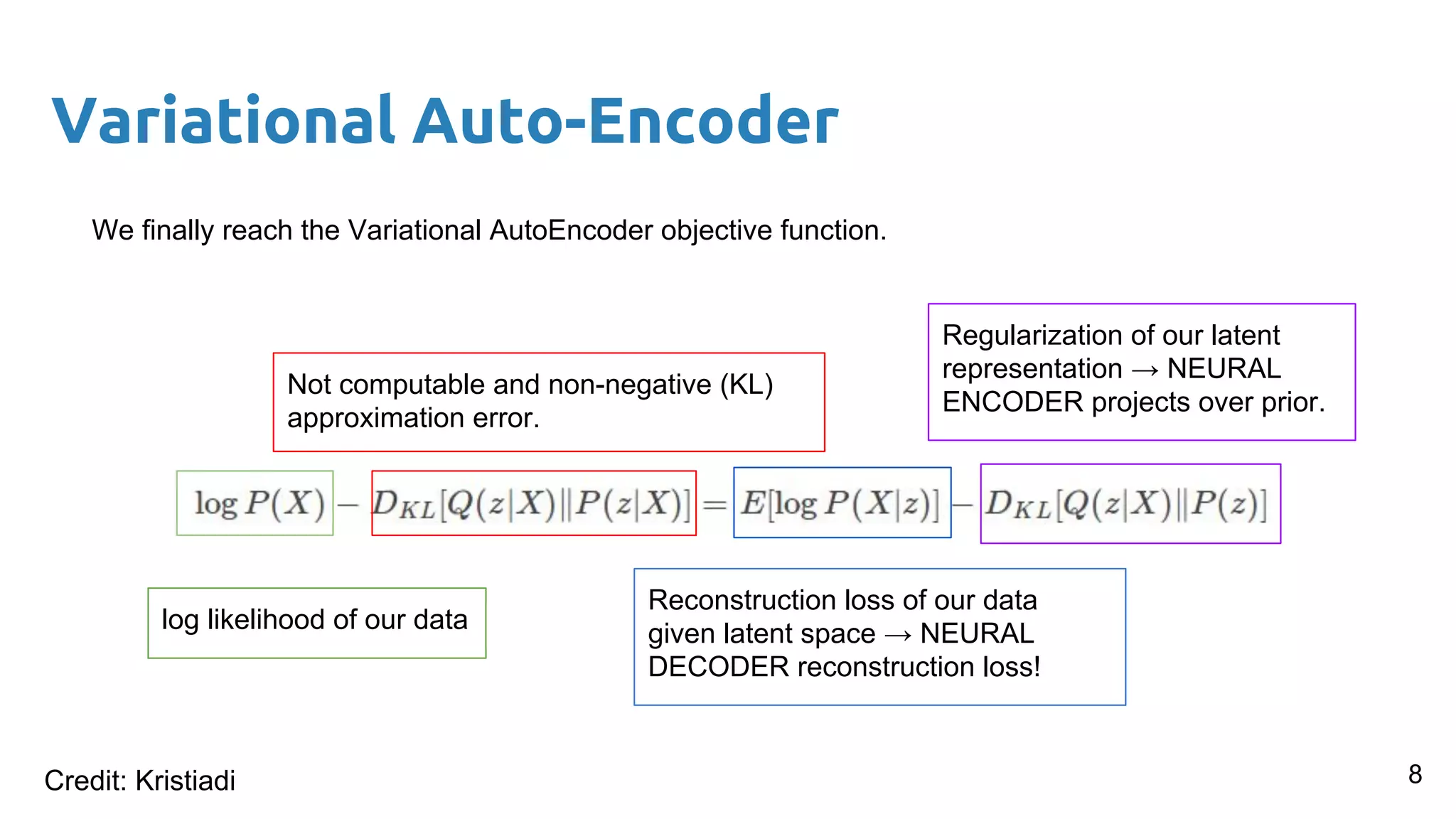
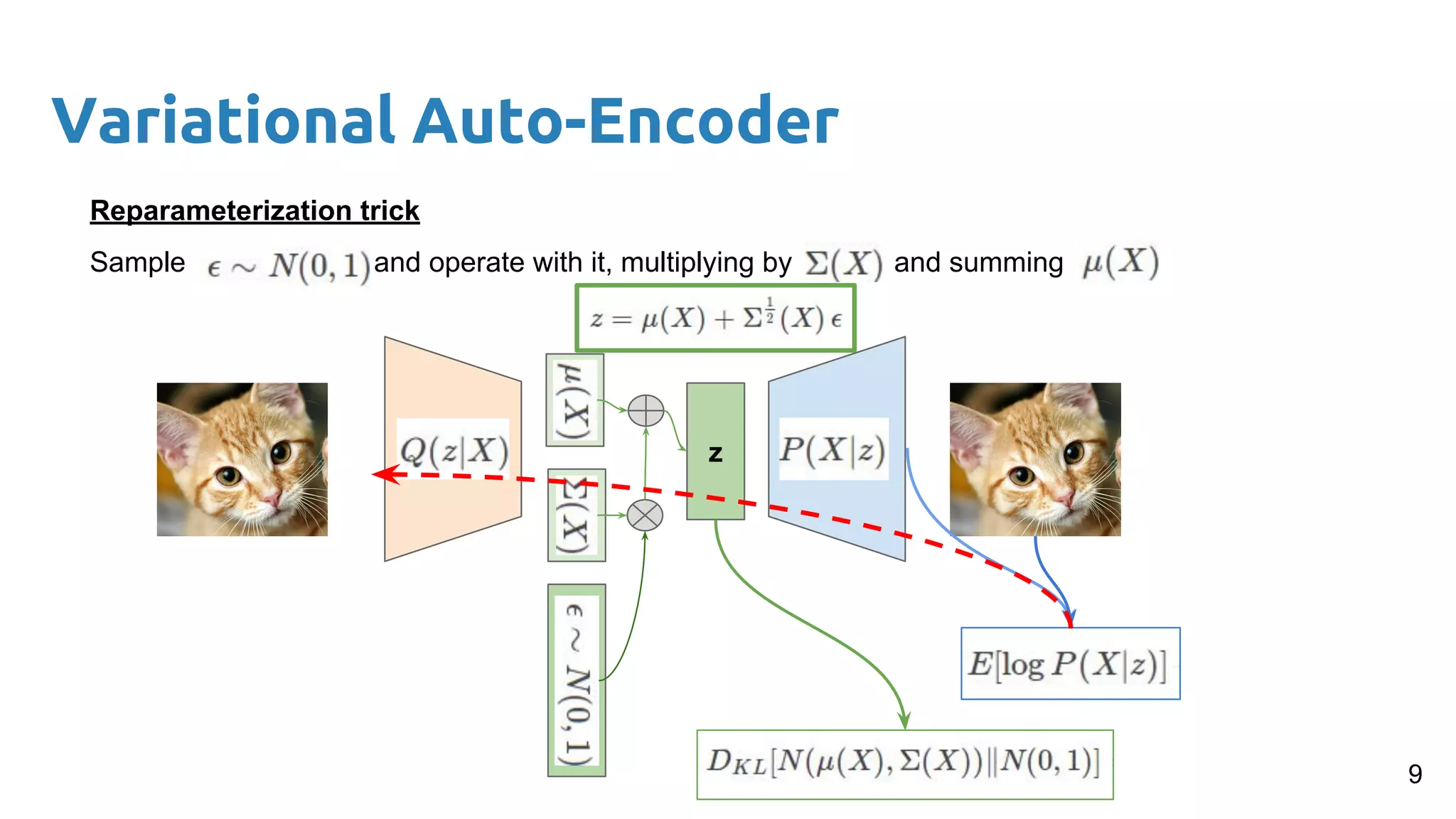
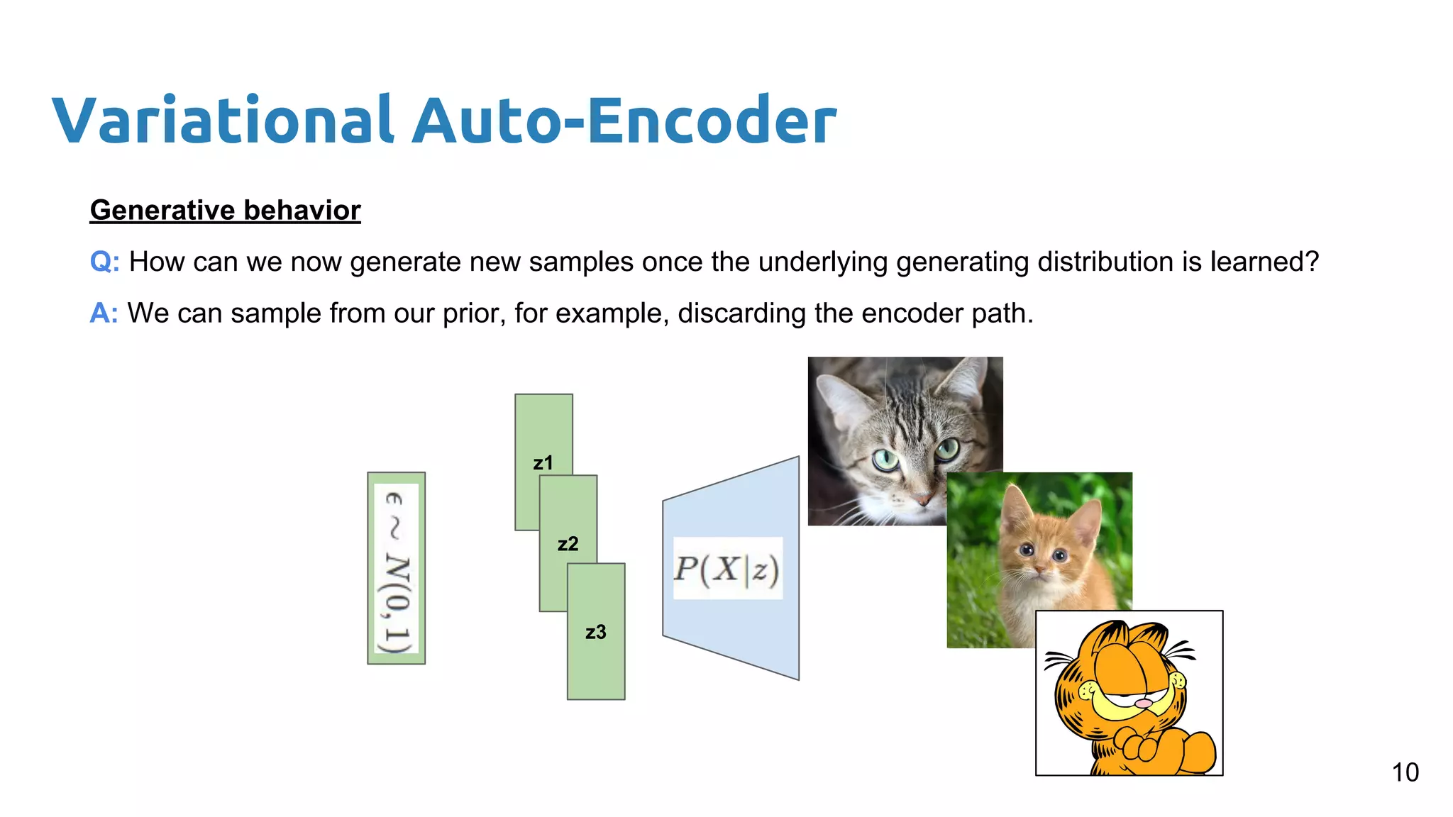
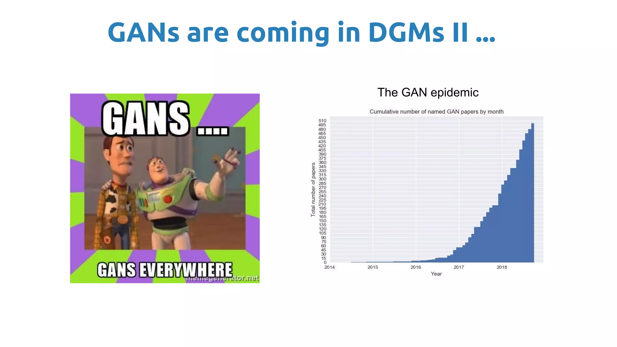
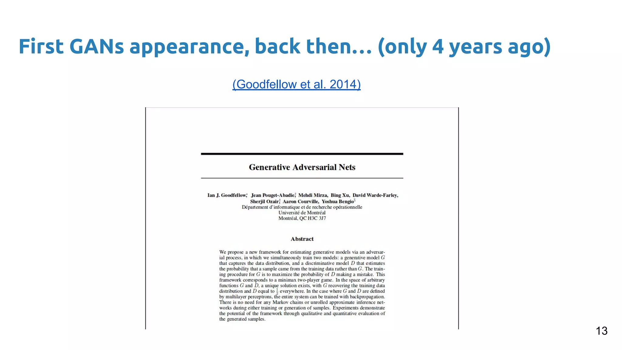
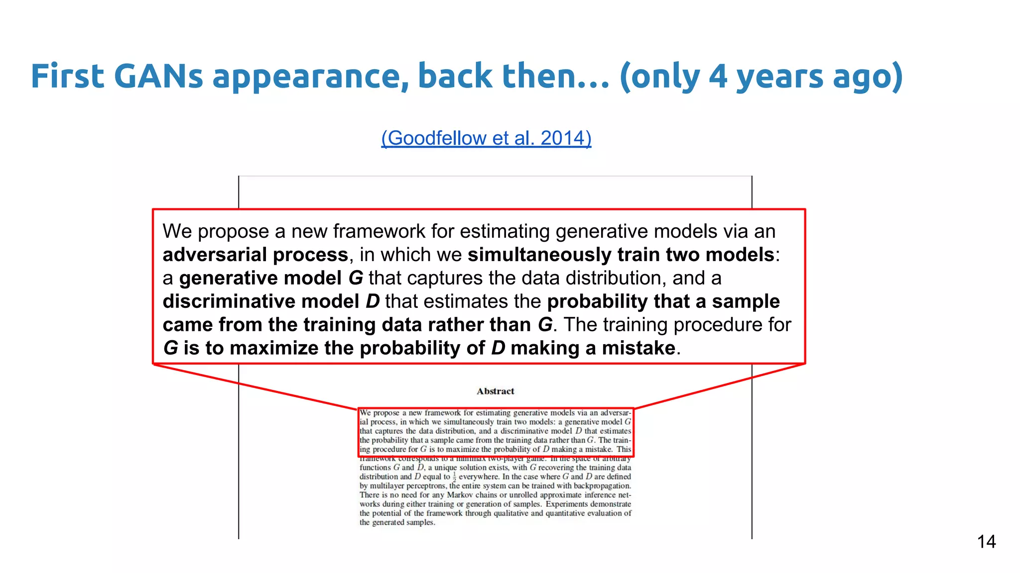
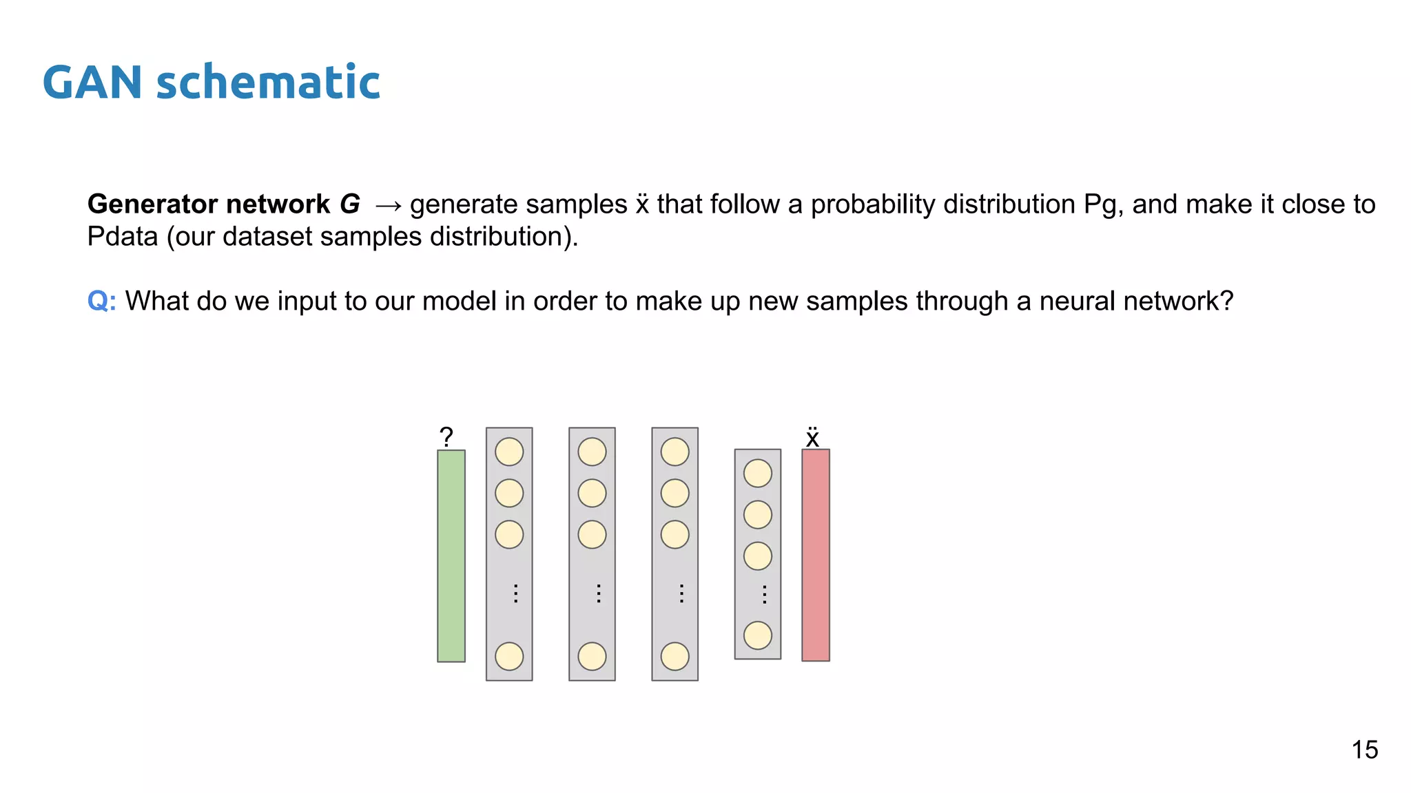
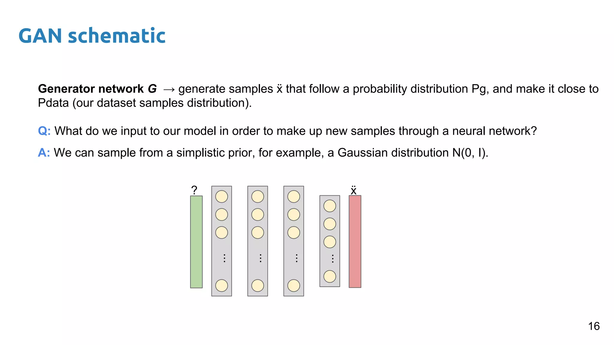
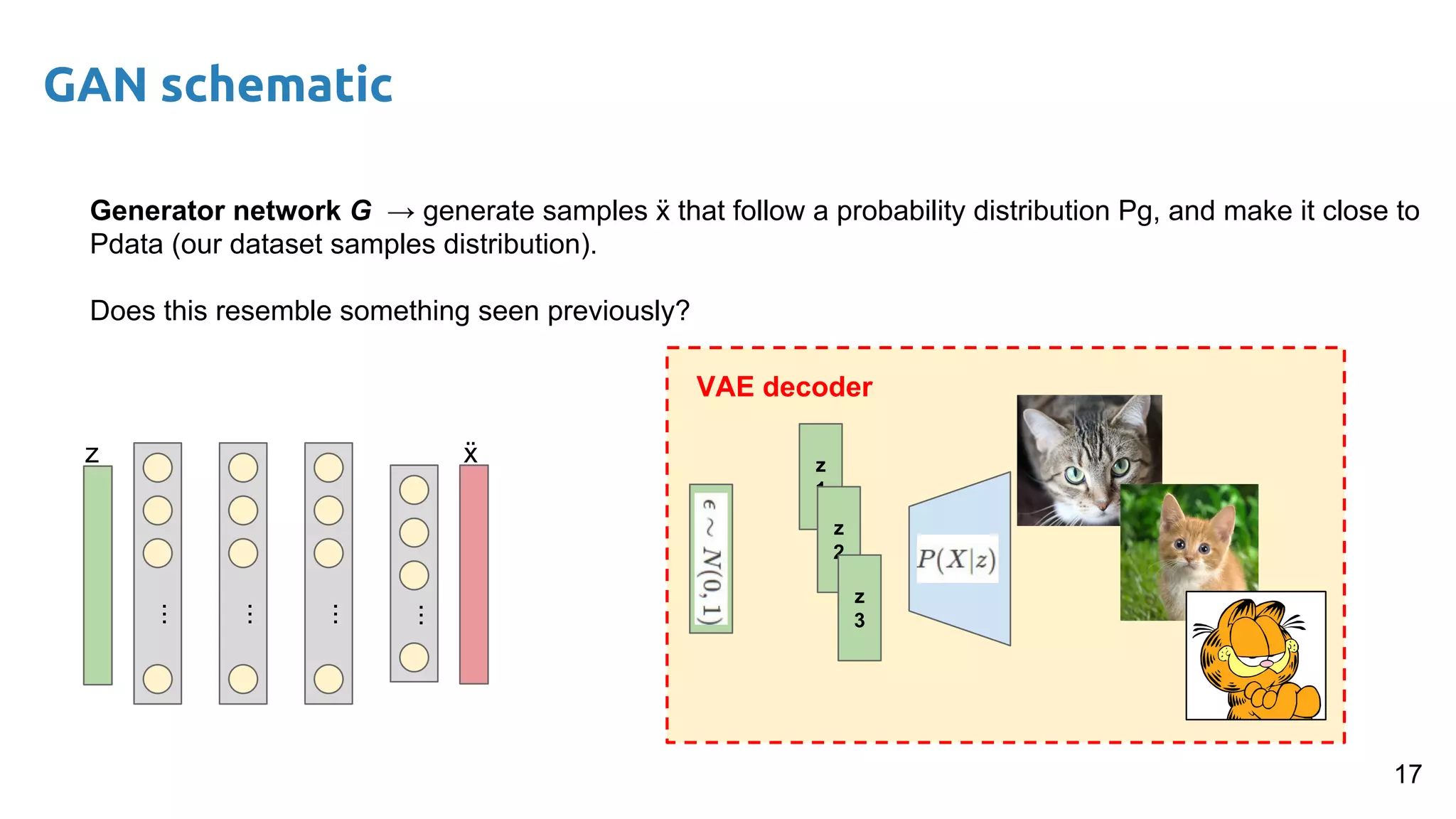
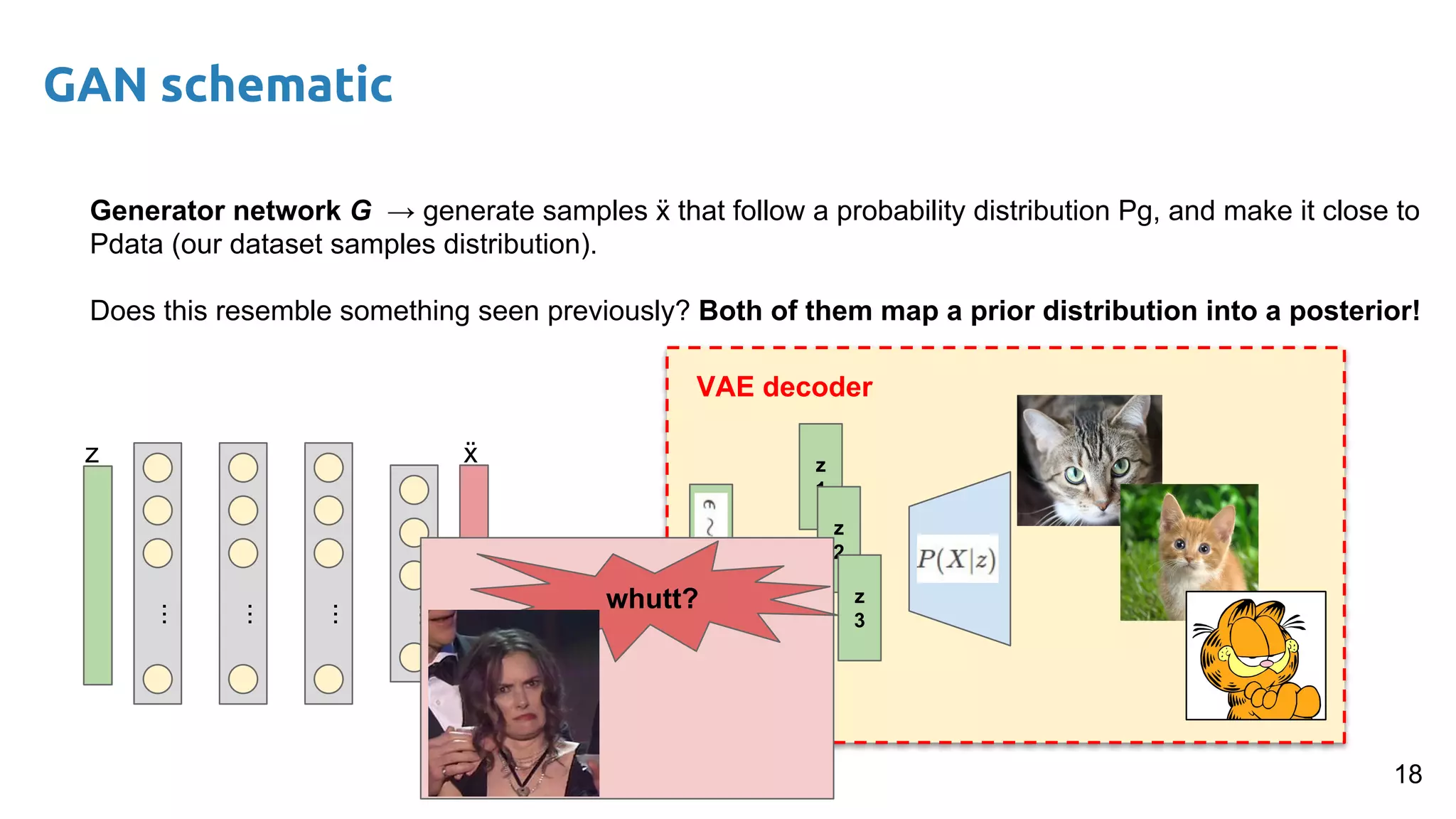
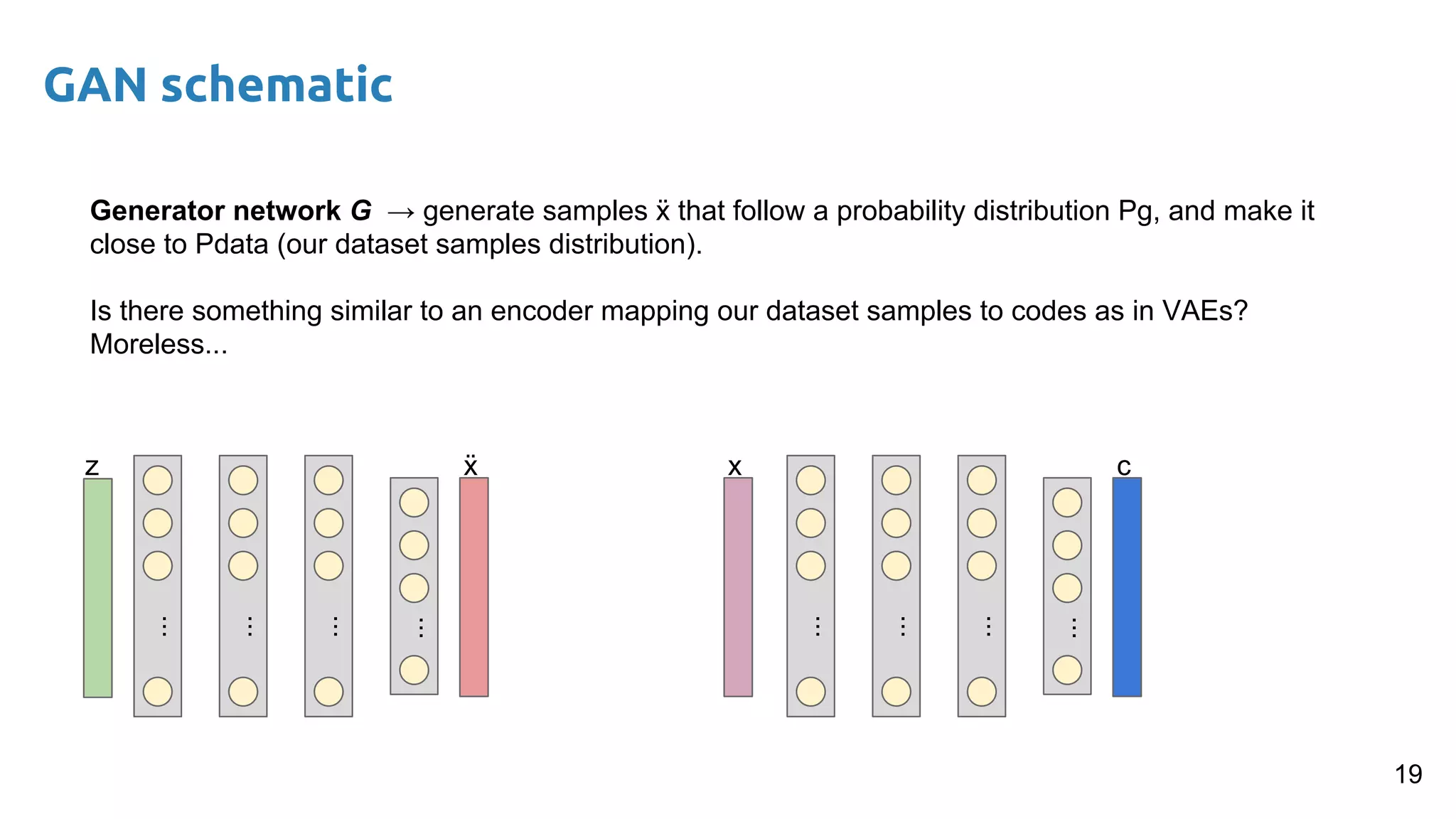
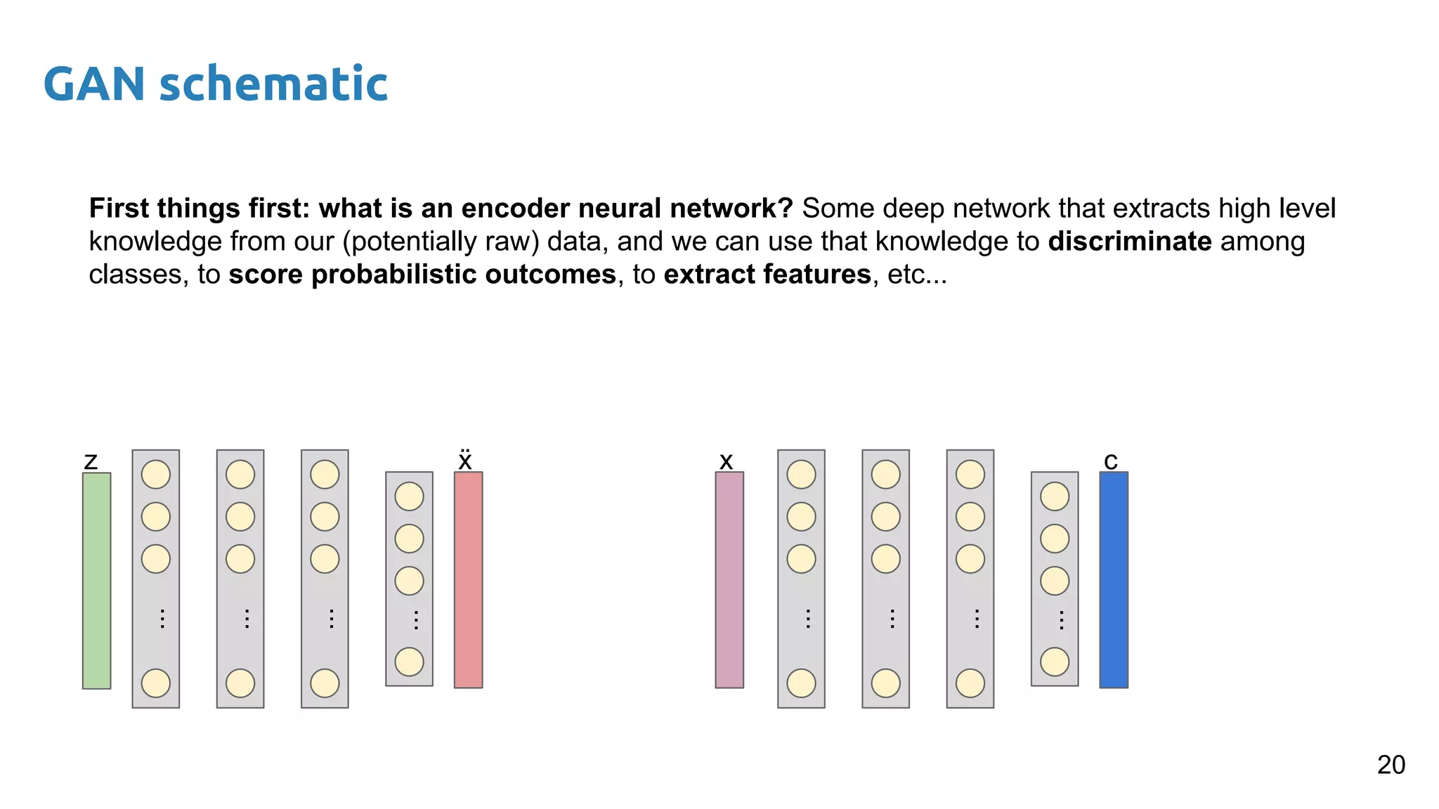
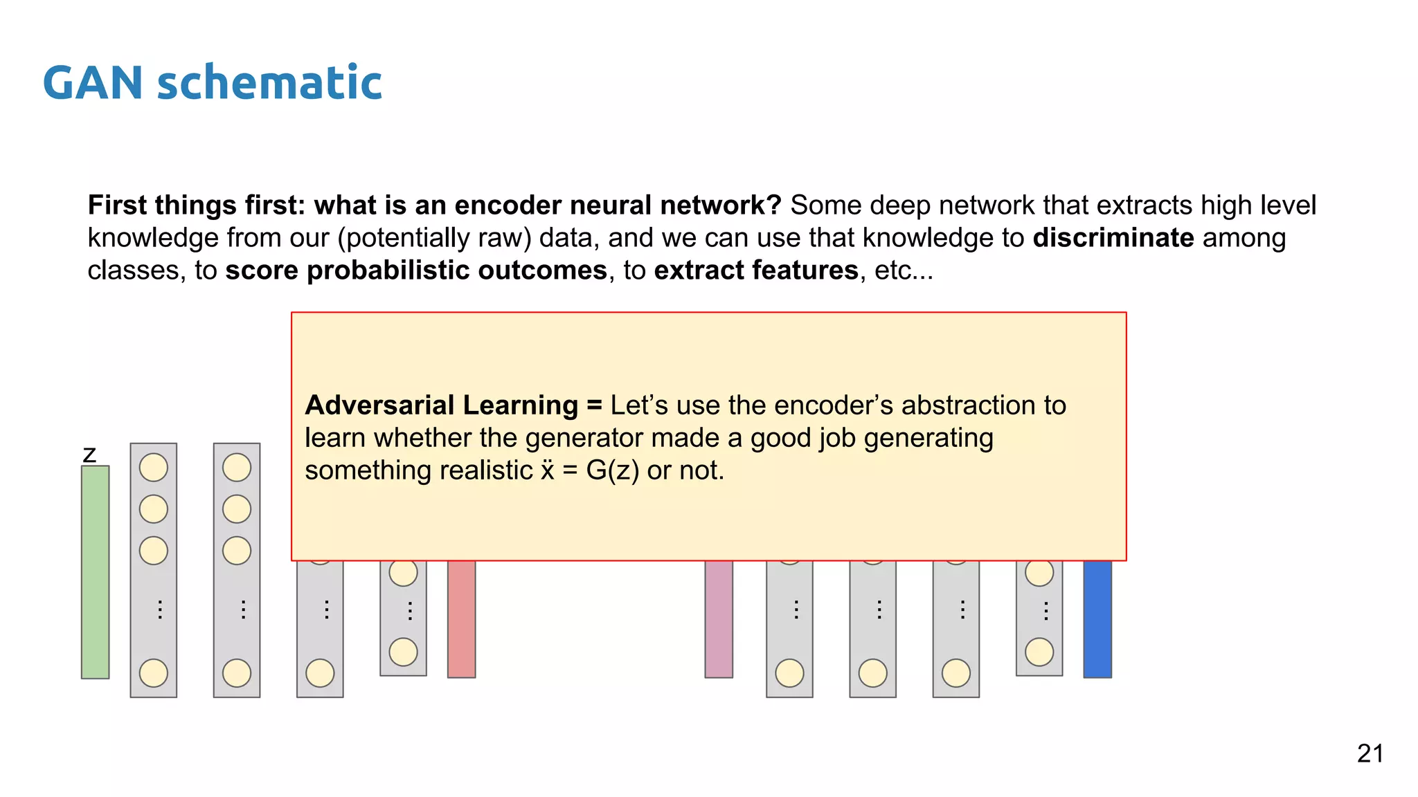
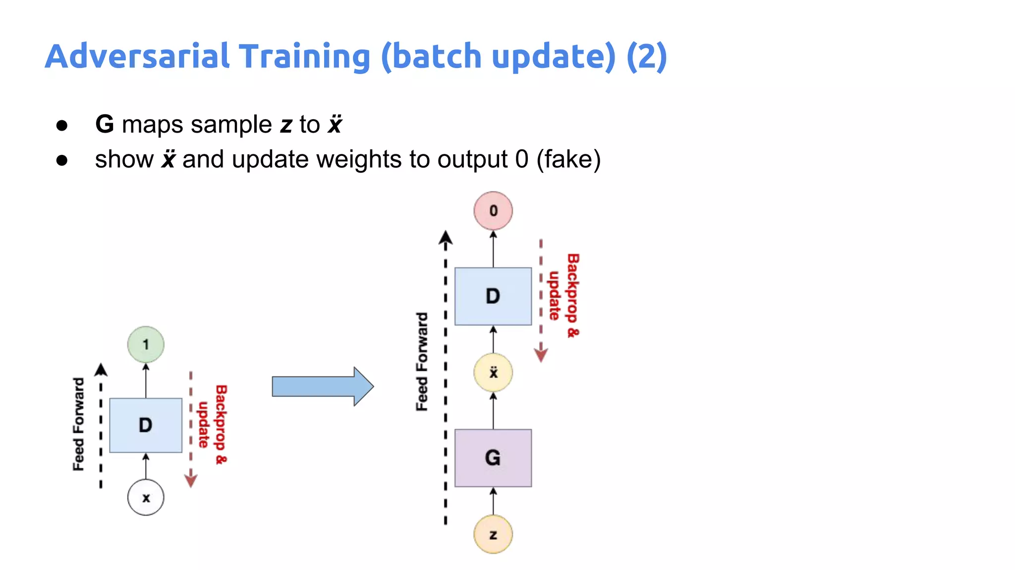
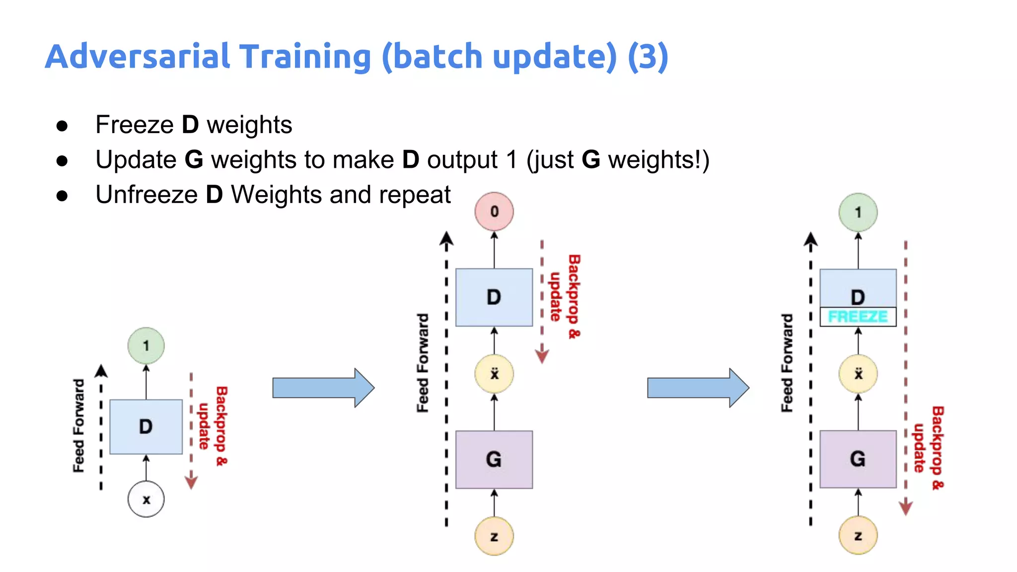
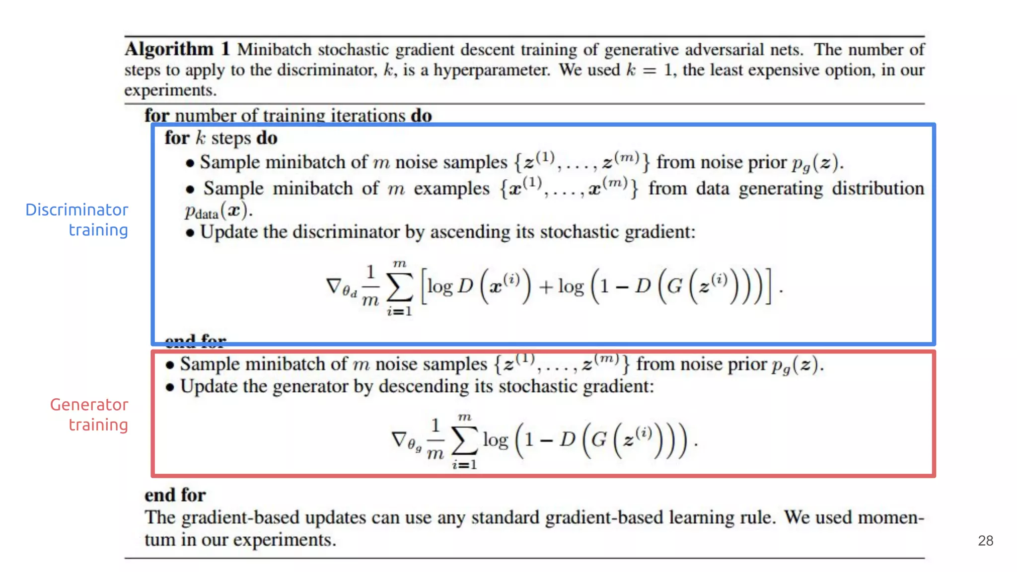
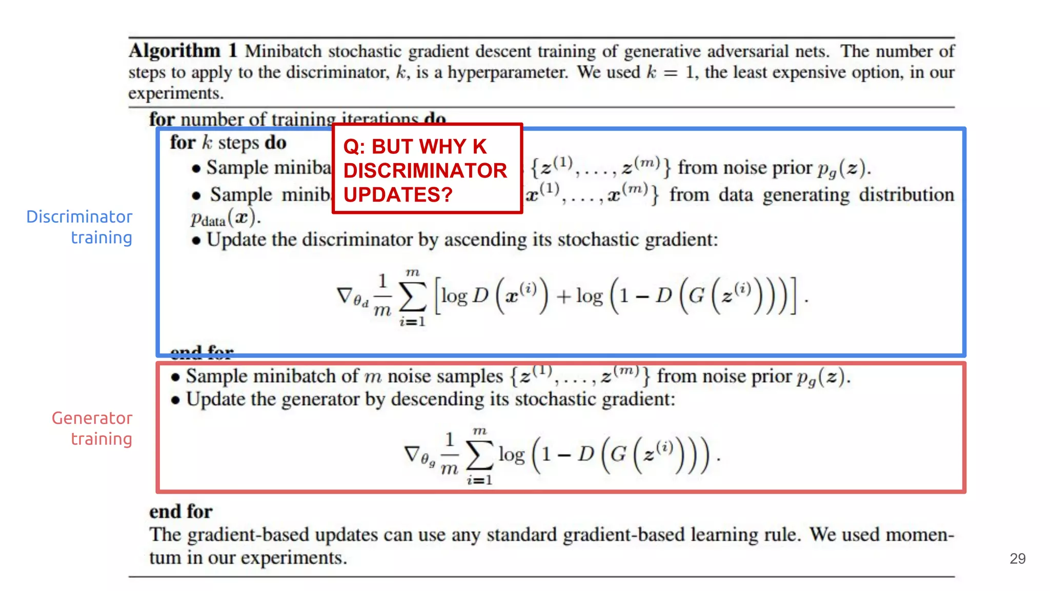
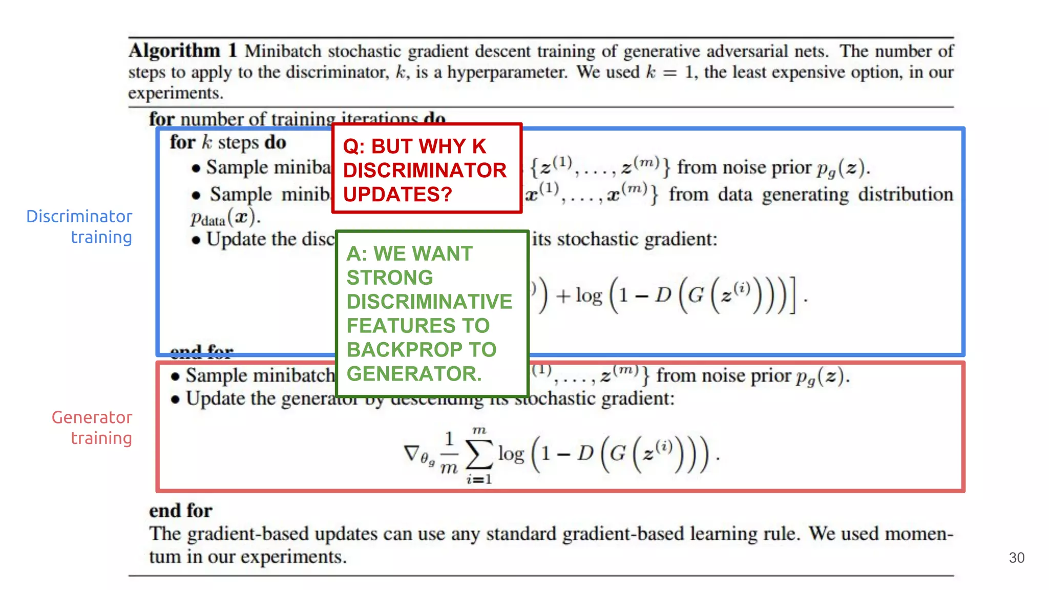
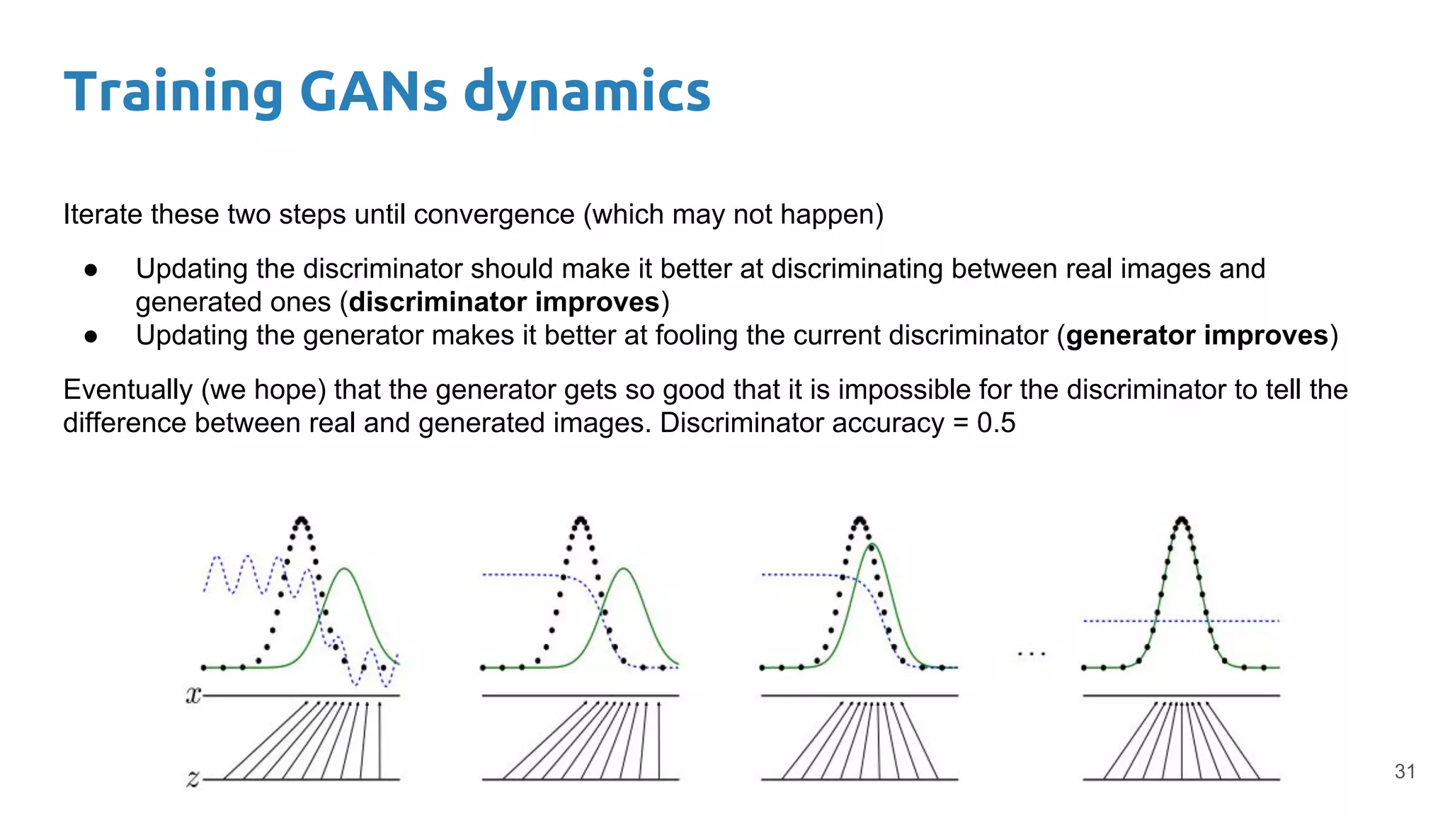
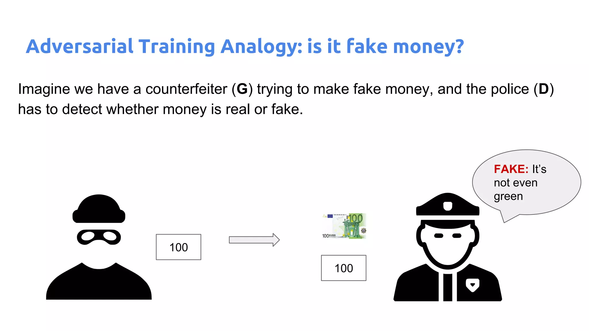
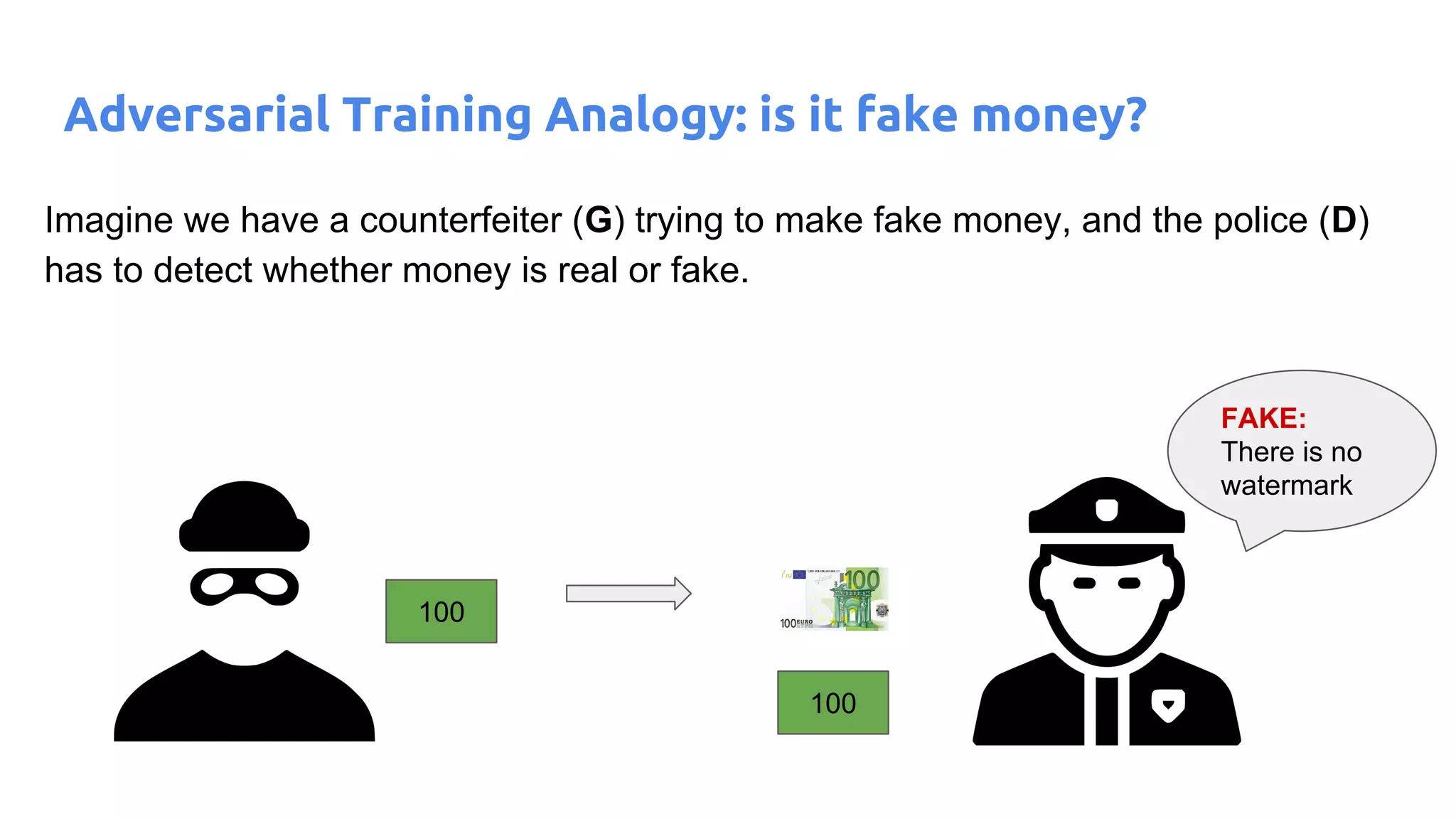
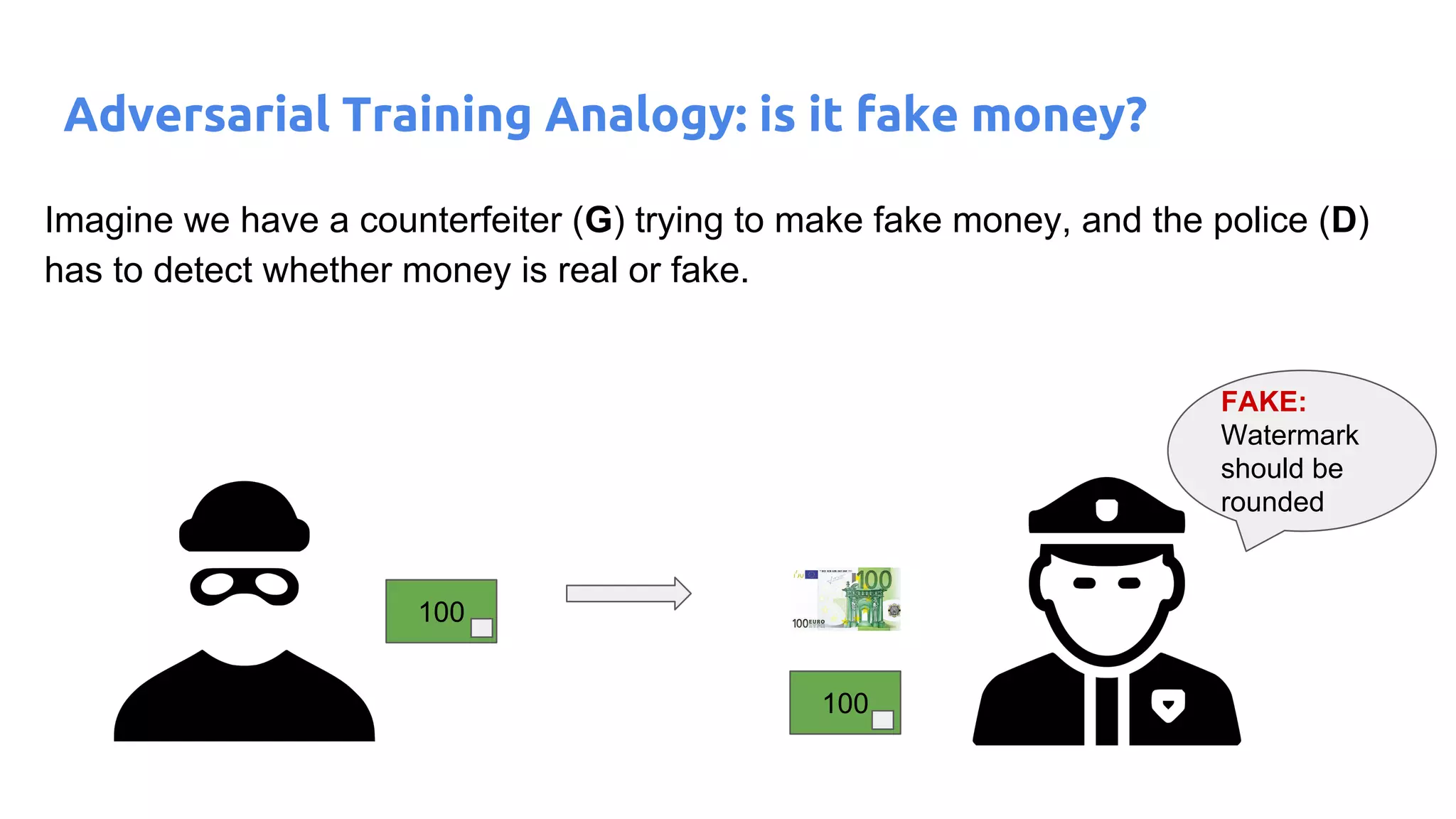
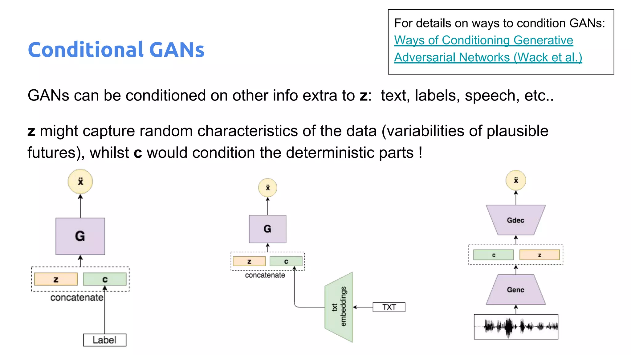
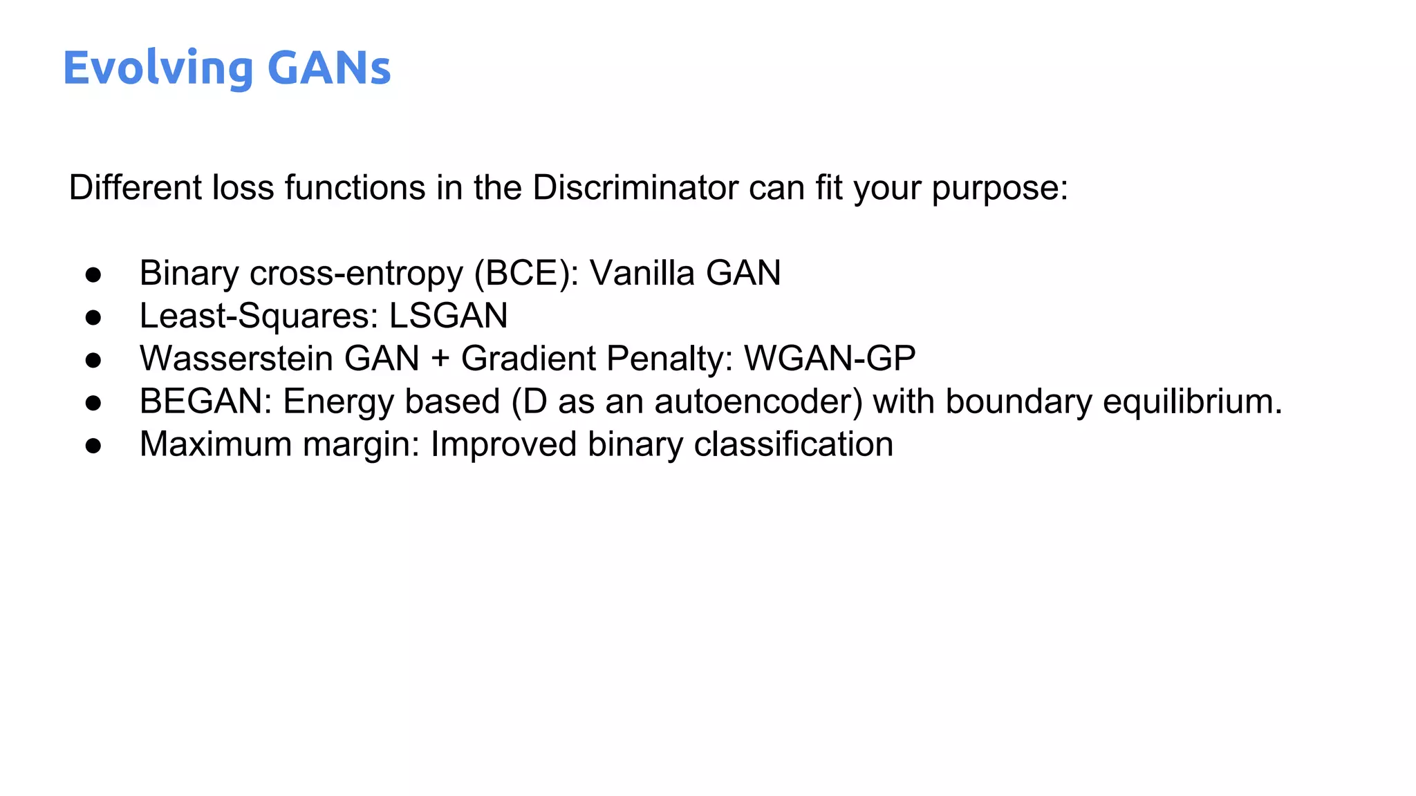
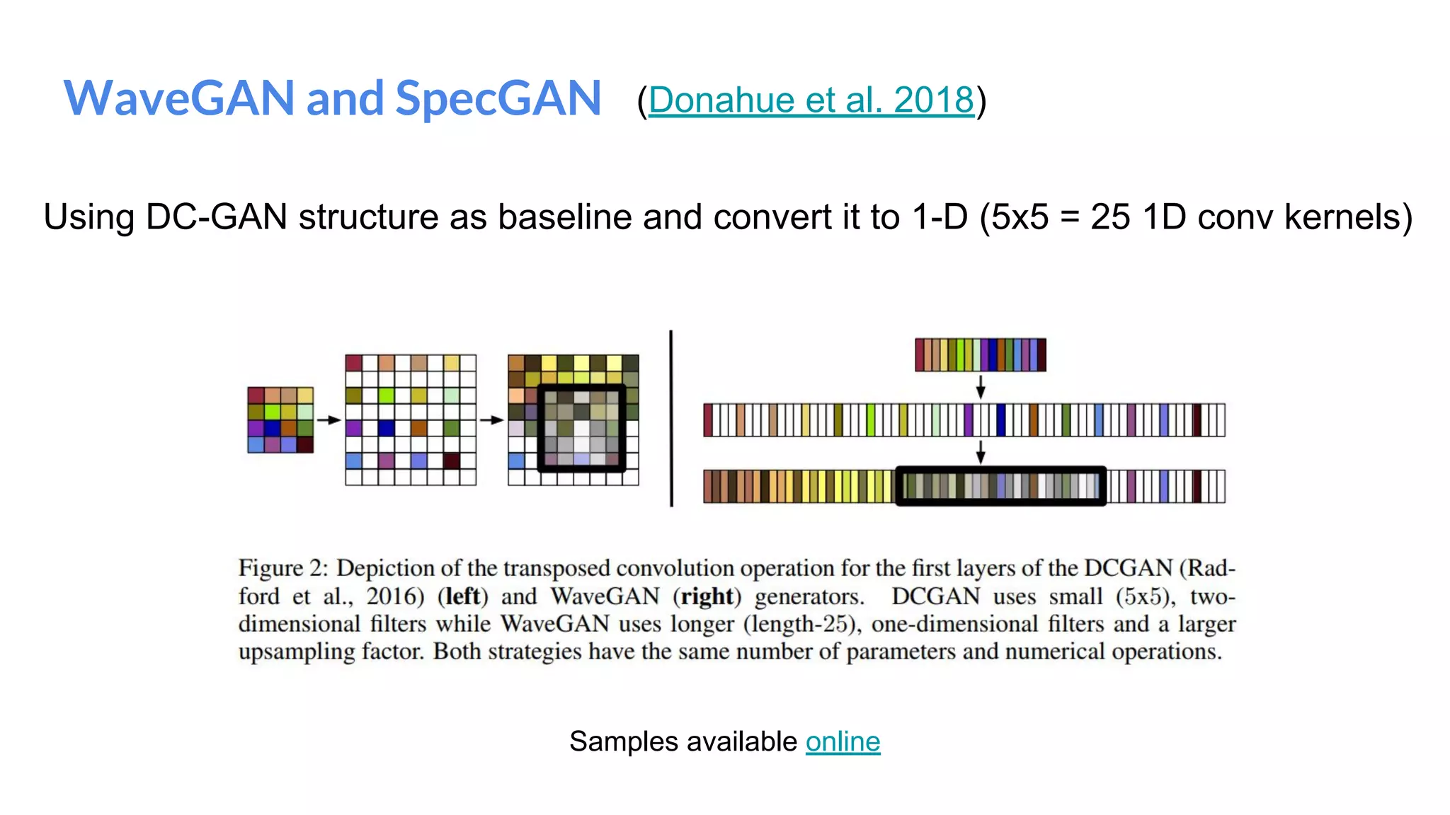
Santiago Pascual de la Puente
santi.pascual@upc.edu
PhD Candidate
Universitat Politecnica de Catalunya
Technical University of Catalonia
Deep Generative Models II
Generative Adversarial Networks
#DLUPC
http://bit.ly/dlai2018
Outline
● What is in here?
● Introduction
● Taxonomy
● Variational Auto-Encoders (VAEs) (DGMs I)
● Generative Adversarial Networks (GANs) (DGMs II)
● PixelCNN/Wavenet
● Normalizing Flows (and flow-based gen. models)
○ Real NVP
○ GLOW
● Models comparison
● Conclusions
2
Previously in DGMs...
What is a generative model?
4
We have datapoints that emerge from some
generating process (landscapes in the nature,
speech from people, etc.)
X = {x1
, x2
, …, xN
}
Having our dataset X with example datapoints
(images, waveforms, written text, etc.) each point xn
lays in some M-dimensional space.
Each point xn
comes from an M-dimensional
probability distribution P(X) → Model it!
5
We can generate any type of data, like speech waveform samples or image pixels.
What is a generative model?
M samples = M dimensions
32
32
.
.
.
Scan and unroll
x3 channels
M = 32x32x3 = 3072 dimensions
Our learned model should be able to make up new samples from the
distribution, not just copy and paste existing samples!
6
What is a generative model?
Figure from NIPS 2016 Tutorial: Generative Adversarial Networks (I. Goodfellow)
7
We will see models that learn the probability density function:
● Explicitly (we impose a known loss function)
○ (1) With approximate density → Variational
Auto-Encoders (VAEs)
○ (2) With tractable density & likelihood-based:
■ PixelCNN, Wavenet.
■ Flow-based models: real-NVP, GLOW.
● Implicitly (we “do not know” the loss function)
○ (3) Generative Adversarial Networks (GANs).
Taxonomy
Variational Auto-Encoder
We finally reach the Variational AutoEncoder objective function.
log likelihood of our data
Not computable and non-negative (KL)
approximation error.
Reconstruction loss of our data
given latent space → NEURAL
DECODER reconstruction loss!
Regularization of our latent
representation → NEURAL
ENCODER projects over prior.
8Credit: Kristiadi
Variational Auto-Encoder
z
Reparameterization trick
Sample and operate with it, multiplying by and summing
9
Variational Auto-Encoder
z1
Generative behavior
Q: How can we now generate new samples once the underlying generating distribution is learned?
A: We can sample from our prior, for example, discarding the encoder path.
z2
z3
10
GANs are coming in DGMs II ...
The GAN epidemic
Generative Adversarial Networks
First GANs appearance, back then… (only 4 years ago)
13
(Goodfellow et al. 2014)
First GANs appearance, back then… (only 4 years ago)
14
(Goodfellow et al. 2014)
We propose a new framework for estimating generative models via an
adversarial process, in which we simultaneously train two models:
a generative model G that captures the data distribution, and a
discriminative model D that estimates the probability that a sample
came from the training data rather than G. The training procedure for
G is to maximize the probability of D making a mistake.
GAN schematic
15
Generator network G → generate samples ẍ that follow a probability distribution Pg, and make it close to
Pdata (our dataset samples distribution).
Q: What do we input to our model in order to make up new samples through a neural network?
...
...
...
...
ẍ?
GAN schematic
16
Generator network G → generate samples ẍ that follow a probability distribution Pg, and make it close to
Pdata (our dataset samples distribution).
Q: What do we input to our model in order to make up new samples through a neural network?
A: We can sample from a simplistic prior, for example, a Gaussian distribution N(0, I).
...
...
...
...
ẍ?
GAN schematic
17
Generator network G → generate samples ẍ that follow a probability distribution Pg, and make it close to
Pdata (our dataset samples distribution).
Does this resemble something seen previously?
...
...
...
...
ẍz z
1
z
2
z
3
VAE decoder
GAN schematic
18
Generator network G → generate samples ẍ that follow a probability distribution Pg, and make it close to
Pdata (our dataset samples distribution).
Does this resemble something seen previously? Both of them map a prior distribution into a posterior!
...
...
...
...
ẍz z
1
z
2
z
3
VAE decoder
whutt?
GAN schematic
19
Generator network G → generate samples ẍ that follow a probability distribution Pg, and make it
close to Pdata (our dataset samples distribution).
Is there something similar to an encoder mapping our dataset samples to codes as in VAEs?
Moreless...
...
...
...
...
ẍz
...
...
...
...
cx
GAN schematic
20
First things first: what is an encoder neural network? Some deep network that extracts high level
knowledge from our (potentially raw) data, and we can use that knowledge to discriminate among
classes, to score probabilistic outcomes, to extract features, etc...
...
...
...
...
ẍz
...
...
...
...
cx
GAN schematic
21
First things first: what is an encoder neural network? Some deep network that extracts high level
knowledge from our (potentially raw) data, and we can use that knowledge to discriminate among
classes, to score probabilistic outcomes, to extract features, etc...
...
...
...
...
ẍz
...
...
...
...
cx
Adversarial Learning = Let’s use the encoder’s abstraction to
learn whether the generator made a good job generating
something realistic ẍ = G(z) or not.
22
Generative + Adversarial
We have two modules: Generator (G) and Discriminator (D).
● They “fight” against each other during training→ Adversarial Learning
● G mission: Fool D to missclassify.
● D mission: Discriminate between G samples and real samples.
Generator
Real world
samples
Database
Discriminator
Real
Loss
Latentrandomvariable
Sample
Sample
Fake
23
z
D is a binary classifier, whose objectives
are: database images are Real, whereas
generated ones are Fake .
Generative + Adversarial
24
We have networks G and D, and training set with pdf Pdata. Notation:
● θ(G), θ(D) (Parameters of model G and D respectively)
● x ~ Pdata (M-dim sample from training data pdf)
● z ~ N(0, I) (sample from prior pdf, e.g. N-dim normal)
● G(z) = ẍ ~ Pmodel (M-dim sample from G network)
D network receives x or ẍ inputs → decides whether input is real or fake. It is optimized to learn: x is real
(1), ẍ is fake (0) (binary classifier).
G network maps sample z to G(z) = ẍ → it is optimized to maximize D mistakes.
NIPS 2016 Tutorial: Generative Adversarial Networks. Ian Goodfellow
Formulations
Adversarial Training (batch update) (1)
● Pick a sample x from training set
● Show x to D and update weights to
output 1 (real)
Adversarial Training (batch update) (2)
● G maps sample z to ẍ
● show ẍ and update weights to output 0 (fake)
Adversarial Training (batch update) (3)
● Freeze D weights
● Update G weights to make D output 1 (just G weights!)
● Unfreeze D Weights and repeat
Discriminator
training
Generator
training
28
Discriminator
training
Generator
training
29
Q: BUT WHY K
DISCRIMINATOR
UPDATES?
Discriminator
training
Generator
training
30
Q: BUT WHY K
DISCRIMINATOR
UPDATES?
A: WE WANT
STRONG
DISCRIMINATIVE
FEATURES TO
BACKPROP TO
GENERATOR.
Training GANs dynamics
Iterate these two steps until convergence (which may not happen)
● Updating the discriminator should make it better at discriminating between real images and
generated ones (discriminator improves)
● Updating the generator makes it better at fooling the current discriminator (generator improves)
Eventually (we hope) that the generator gets so good that it is impossible for the discriminator to tell the
difference between real and generated images. Discriminator accuracy = 0.5
31
Adversarial Training Analogy: is it fake money?
Imagine we have a counterfeiter (G) trying to make fake money, and the police (D)
has to detect whether money is real or fake.
Key Idea: D is trained to detect fraud, (its parameters learn discriminative features
of “what is real/fake”). As backprop goes through D to G there happens to be
information leaking about the requirements for bank notes to look real. This makes
G perform small corrections to get closer and closer to what real samples would be.
Caveat: this means GANs are not suitable for discrete
tokens predictions (e.g. words) → in that discrete space
there is no “small change” criteria to get to a neighbour (but can
work in a word embedding space for example).
Adversarial Training Analogy: is it fake money?
Imagine we have a counterfeiter (G) trying to make fake money, and the police (D)
has to detect whether money is real or fake.
100
100
FAKE: It’s
not even
green
Adversarial Training Analogy: is it fake money?
Imagine we have a counterfeiter (G) trying to make fake money, and the police (D)
has to detect whether money is real or fake.
100
100
FAKE:
There is no
watermark
Adversarial Training Analogy: is it fake money?
Imagine we have a counterfeiter (G) trying to make fake money, and the police (D)
has to detect whether money is real or fake.
100
100
FAKE:
Watermark
should be
rounded
Adversarial Training Analogy: is it fake money?
Imagine we have a counterfeiter (G) trying to make fake money, and the police (D)
has to detect whether money is real or fake.
After enough iterations, and if the counterfeiter is good enough (in terms of G
network it means “has enough parameters”), the police should be confused.
REAL?
FAKE?
Adversarial Training Analogy: is it fake money?
Conditional GANs
GANs can be conditioned on other info extra to z:
text, labels, speech, etc..
z might capture random characteristics of the data
(variabilities of plausible futures), whilst c would
condition the deterministic parts !
For details on ways to condition GANs:
Ways of Conditioning Generative
Adversarial Networks (Wack et al.)
Conditional GANs
GANs can be conditioned on other info extra to z: text, labels, speech, etc..
z might capture random characteristics of the data (variabilities of plausible
futures), whilst c would condition the deterministic parts !
For details on ways to condition GANs:
Ways of Conditioning Generative
Adversarial Networks (Wack et al.)
Where is the downside...?
GANs are tricky and hard to train! We do not want to minimize a cost function.
Instead we want both networks to reach Nash equilibria (saddle point).
● Formulated as a “game” between two networks
● Unstable dynamics: hard to keep generator and discriminator in balance
● Optimization can oscillate between solutions
● Generator can collapse (generate low variability at its output)
Caveats
Where is the downside...?
GANs are tricky and hard to train! We do not want to minimize a cost function.
Instead we want both networks to reach Nash equilibria (saddle point).
Caveats
Because of extensive experience within the GAN community (with some
does-not-work-frustration from time to time), you can find some tricks and
tips on how to train a vanilla GAN here:
https://github.com/soumith/ganhacks
Evolving GANs
Different loss functions in the Discriminator can fit your purpose:
● Binary cross-entropy (BCE): Vanilla GAN
● Least-Squares: LSGAN
● Wasserstein GAN + Gradient Penalty: WGAN-GP
● BEGAN: Energy based (D as an autoencoder) with boundary equilibrium.
● Maximum margin: Improved binary classification
Least Squares GAN
Main idea: shift to loss function that provides smooth & non-saturating gradients in D
● Because of sigmoid saturation in binary classification loss, G gets no info when
D gets to label true examples → vanishing gradients make G no learn
● Least squares loss improves learning with notion of distance of Pmodel to Pdata:
Least Squares Generative Adversarial
Networks, Mao et al. 2016
Other GAN implementations
Other GAN implementations try to stabilize learning dynamics, imposing new
divergences to be measured by D → gradients flow better and loss gets correlated
with generation quality:
● Wasserstein GAN (Arjovsky et al. 2017)
● BEGAN: Boundary Equilibrium Generative Adversarial Networks (Berthelot et al. 2017)
● WGAN-GP: Improved Training of Wasserstein GANs (Gulrajani et al. 2017)
Bi-GAN (Bidirectional) (Donahue et al. 2016)
Learn both mappings, ẍ = G(z) and ẑ = E(x) simultaneously. This allows us to perform arithmetics in
Z space without using any iterative gradient ascent algorithm to find the z matching some x, we rather
forward through encoder E.
Generating images/frames
(Radford et al. 2015)
Deep Conv. GAN (DCGAN) effectively generated 64x64 RGB images in a single
shot. It is also the base of all image generation GAN architectures.
fully
connected Strided
transposed
conv layers
Conv layers,
no max-pool
fully
connected
Generating images/frames conditioned on captions
Generative Adversarial Text to Image Synthesis (Reed et al. 2016b)
Generating images/frames conditioned on captions
StackGAN (Zhang et al. 2016). Increased resolution to 256x256,
conceptual two-stage: ‘Draft’ and ‘Fine-grained detalis’
Generating images/frames conditioned on captions
(Reed et al. 2016b) (Zhang et al. 2016)
Unsupervised feature extraction/learning representations
Similarly to word2vec, GANs learn a distributed representation that disentangles
concepts such that we can perform semantic operations on the data manifold:
v(Man with glasses) - v(man) + v(woman) = v(woman with glasses)
(Radford et al. 2015)
Image super-resolution
Bicubic: not using data statistics. SRResNet: trained with MSE. SRGAN is able to
understand that there are multiple correct answers, rather than averaging.
(Ledig et al. 2016)
Image super-resolution
Averaging is a serious problem we face when dealing with complex distributions.
(Ledig et al. 2016)
53
DCGAN Imagenet conditional generation (2016)
(Goodfellow 2016)
“Old” results with 128x128
imagenet generated images.
Global structure is lost, and
training requires many tweaks
(GANHacks 2016).
54
Self-Attention GAN (Zhang et al. 2018)
Self-Attention GAN
55
Self-Attention GAN Imagenet conditional generation (2018)
New May 2018 state of the art
results with 128x128 imagenet
generated images. Global
structure is now preserved and
GANs traing more stable.
(Zhang et al. 2018)
56
Big GAN (2018)
Current (Oct 2018) state of the
art results with 512x512
imagenet generated images!
(Brock et al. 2018)
Speech Enhancement
Speech Enhancement GAN (Pascual et al. 2017)
Speech Enhancement
Samples available here
Code available here
WaveGAN and SpecGAN (Donahue et al. 2018)
Using DC-GAN structure as baseline and convert it to 1-D (5x5 = 25 1D conv kernels)
Samples available online
Thanks! Questions?

Generative Adversarial Networks GAN - Santiago Pascual - UPC Barcelona 2018

  • 1.
    Santiago Pascual dela Puente santi.pascual@upc.edu PhD Candidate Universitat Politecnica de Catalunya Technical University of Catalonia Deep Generative Models II Generative Adversarial Networks #DLUPC http://bit.ly/dlai2018
  • 2.
    Outline ● What isin here? ● Introduction ● Taxonomy ● Variational Auto-Encoders (VAEs) (DGMs I) ● Generative Adversarial Networks (GANs) (DGMs II) ● PixelCNN/Wavenet ● Normalizing Flows (and flow-based gen. models) ○ Real NVP ○ GLOW ● Models comparison ● Conclusions 2
  • 3.
  • 4.
    What is agenerative model? 4 We have datapoints that emerge from some generating process (landscapes in the nature, speech from people, etc.) X = {x1 , x2 , …, xN } Having our dataset X with example datapoints (images, waveforms, written text, etc.) each point xn lays in some M-dimensional space. Each point xn comes from an M-dimensional probability distribution P(X) → Model it!
  • 5.
    5 We can generateany type of data, like speech waveform samples or image pixels. What is a generative model? M samples = M dimensions 32 32 . . . Scan and unroll x3 channels M = 32x32x3 = 3072 dimensions
  • 6.
    Our learned modelshould be able to make up new samples from the distribution, not just copy and paste existing samples! 6 What is a generative model? Figure from NIPS 2016 Tutorial: Generative Adversarial Networks (I. Goodfellow)
  • 7.
    7 We will seemodels that learn the probability density function: ● Explicitly (we impose a known loss function) ○ (1) With approximate density → Variational Auto-Encoders (VAEs) ○ (2) With tractable density & likelihood-based: ■ PixelCNN, Wavenet. ■ Flow-based models: real-NVP, GLOW. ● Implicitly (we “do not know” the loss function) ○ (3) Generative Adversarial Networks (GANs). Taxonomy
  • 8.
    Variational Auto-Encoder We finallyreach the Variational AutoEncoder objective function. log likelihood of our data Not computable and non-negative (KL) approximation error. Reconstruction loss of our data given latent space → NEURAL DECODER reconstruction loss! Regularization of our latent representation → NEURAL ENCODER projects over prior. 8Credit: Kristiadi
  • 9.
    Variational Auto-Encoder z Reparameterization trick Sampleand operate with it, multiplying by and summing 9
  • 10.
    Variational Auto-Encoder z1 Generative behavior Q:How can we now generate new samples once the underlying generating distribution is learned? A: We can sample from our prior, for example, discarding the encoder path. z2 z3 10
  • 11.
    GANs are comingin DGMs II ... The GAN epidemic
  • 12.
  • 13.
    First GANs appearance,back then… (only 4 years ago) 13 (Goodfellow et al. 2014)
  • 14.
    First GANs appearance,back then… (only 4 years ago) 14 (Goodfellow et al. 2014) We propose a new framework for estimating generative models via an adversarial process, in which we simultaneously train two models: a generative model G that captures the data distribution, and a discriminative model D that estimates the probability that a sample came from the training data rather than G. The training procedure for G is to maximize the probability of D making a mistake.
  • 15.
    GAN schematic 15 Generator networkG → generate samples ẍ that follow a probability distribution Pg, and make it close to Pdata (our dataset samples distribution). Q: What do we input to our model in order to make up new samples through a neural network? ... ... ... ... ẍ?
  • 16.
    GAN schematic 16 Generator networkG → generate samples ẍ that follow a probability distribution Pg, and make it close to Pdata (our dataset samples distribution). Q: What do we input to our model in order to make up new samples through a neural network? A: We can sample from a simplistic prior, for example, a Gaussian distribution N(0, I). ... ... ... ... ẍ?
  • 17.
    GAN schematic 17 Generator networkG → generate samples ẍ that follow a probability distribution Pg, and make it close to Pdata (our dataset samples distribution). Does this resemble something seen previously? ... ... ... ... ẍz z 1 z 2 z 3 VAE decoder
  • 18.
    GAN schematic 18 Generator networkG → generate samples ẍ that follow a probability distribution Pg, and make it close to Pdata (our dataset samples distribution). Does this resemble something seen previously? Both of them map a prior distribution into a posterior! ... ... ... ... ẍz z 1 z 2 z 3 VAE decoder whutt?
  • 19.
    GAN schematic 19 Generator networkG → generate samples ẍ that follow a probability distribution Pg, and make it close to Pdata (our dataset samples distribution). Is there something similar to an encoder mapping our dataset samples to codes as in VAEs? Moreless... ... ... ... ... ẍz ... ... ... ... cx
  • 20.
    GAN schematic 20 First thingsfirst: what is an encoder neural network? Some deep network that extracts high level knowledge from our (potentially raw) data, and we can use that knowledge to discriminate among classes, to score probabilistic outcomes, to extract features, etc... ... ... ... ... ẍz ... ... ... ... cx
  • 21.
    GAN schematic 21 First thingsfirst: what is an encoder neural network? Some deep network that extracts high level knowledge from our (potentially raw) data, and we can use that knowledge to discriminate among classes, to score probabilistic outcomes, to extract features, etc... ... ... ... ... ẍz ... ... ... ... cx Adversarial Learning = Let’s use the encoder’s abstraction to learn whether the generator made a good job generating something realistic ẍ = G(z) or not.
  • 22.
    22 Generative + Adversarial Wehave two modules: Generator (G) and Discriminator (D). ● They “fight” against each other during training→ Adversarial Learning ● G mission: Fool D to missclassify. ● D mission: Discriminate between G samples and real samples.
  • 23.
    Generator Real world samples Database Discriminator Real Loss Latentrandomvariable Sample Sample Fake 23 z D isa binary classifier, whose objectives are: database images are Real, whereas generated ones are Fake . Generative + Adversarial
  • 24.
    24 We have networksG and D, and training set with pdf Pdata. Notation: ● θ(G), θ(D) (Parameters of model G and D respectively) ● x ~ Pdata (M-dim sample from training data pdf) ● z ~ N(0, I) (sample from prior pdf, e.g. N-dim normal) ● G(z) = ẍ ~ Pmodel (M-dim sample from G network) D network receives x or ẍ inputs → decides whether input is real or fake. It is optimized to learn: x is real (1), ẍ is fake (0) (binary classifier). G network maps sample z to G(z) = ẍ → it is optimized to maximize D mistakes. NIPS 2016 Tutorial: Generative Adversarial Networks. Ian Goodfellow Formulations
  • 25.
    Adversarial Training (batchupdate) (1) ● Pick a sample x from training set ● Show x to D and update weights to output 1 (real)
  • 26.
    Adversarial Training (batchupdate) (2) ● G maps sample z to ẍ ● show ẍ and update weights to output 0 (fake)
  • 27.
    Adversarial Training (batchupdate) (3) ● Freeze D weights ● Update G weights to make D output 1 (just G weights!) ● Unfreeze D Weights and repeat
  • 28.
  • 29.
  • 30.
    Discriminator training Generator training 30 Q: BUT WHYK DISCRIMINATOR UPDATES? A: WE WANT STRONG DISCRIMINATIVE FEATURES TO BACKPROP TO GENERATOR.
  • 31.
    Training GANs dynamics Iteratethese two steps until convergence (which may not happen) ● Updating the discriminator should make it better at discriminating between real images and generated ones (discriminator improves) ● Updating the generator makes it better at fooling the current discriminator (generator improves) Eventually (we hope) that the generator gets so good that it is impossible for the discriminator to tell the difference between real and generated images. Discriminator accuracy = 0.5 31
  • 32.
    Adversarial Training Analogy:is it fake money? Imagine we have a counterfeiter (G) trying to make fake money, and the police (D) has to detect whether money is real or fake. Key Idea: D is trained to detect fraud, (its parameters learn discriminative features of “what is real/fake”). As backprop goes through D to G there happens to be information leaking about the requirements for bank notes to look real. This makes G perform small corrections to get closer and closer to what real samples would be.
  • 33.
    Imagine we havea counterfeiter (G) trying to make fake money, and the police (D) has to detect whether money is real or fake. Key Idea: D is trained to detect fraud, (its parameters learn discriminative features of “what is real/fake”). As backprop goes through D to G there happens to be information leaking about the requirements for bank notes to look real. This makes G perform small corrections to get closer and closer to what real samples would be. Caveat: this means GANs are not suitable for discrete tokens predictions (e.g. words) → in that discrete space there is no “small change” criteria to get to a neighbour (but can work in a word embedding space for example). Adversarial Training Analogy: is it fake money?
  • 34.
    Imagine we havea counterfeiter (G) trying to make fake money, and the police (D) has to detect whether money is real or fake. 100 100 FAKE: It’s not even green Adversarial Training Analogy: is it fake money?
  • 35.
    Imagine we havea counterfeiter (G) trying to make fake money, and the police (D) has to detect whether money is real or fake. 100 100 FAKE: There is no watermark Adversarial Training Analogy: is it fake money?
  • 36.
    Imagine we havea counterfeiter (G) trying to make fake money, and the police (D) has to detect whether money is real or fake. 100 100 FAKE: Watermark should be rounded Adversarial Training Analogy: is it fake money?
  • 37.
    Imagine we havea counterfeiter (G) trying to make fake money, and the police (D) has to detect whether money is real or fake. After enough iterations, and if the counterfeiter is good enough (in terms of G network it means “has enough parameters”), the police should be confused. REAL? FAKE? Adversarial Training Analogy: is it fake money?
  • 38.
    Conditional GANs GANs canbe conditioned on other info extra to z: text, labels, speech, etc.. z might capture random characteristics of the data (variabilities of plausible futures), whilst c would condition the deterministic parts ! For details on ways to condition GANs: Ways of Conditioning Generative Adversarial Networks (Wack et al.)
  • 39.
    Conditional GANs GANs canbe conditioned on other info extra to z: text, labels, speech, etc.. z might capture random characteristics of the data (variabilities of plausible futures), whilst c would condition the deterministic parts ! For details on ways to condition GANs: Ways of Conditioning Generative Adversarial Networks (Wack et al.)
  • 40.
    Where is thedownside...? GANs are tricky and hard to train! We do not want to minimize a cost function. Instead we want both networks to reach Nash equilibria (saddle point). ● Formulated as a “game” between two networks ● Unstable dynamics: hard to keep generator and discriminator in balance ● Optimization can oscillate between solutions ● Generator can collapse (generate low variability at its output) Caveats
  • 41.
    Where is thedownside...? GANs are tricky and hard to train! We do not want to minimize a cost function. Instead we want both networks to reach Nash equilibria (saddle point). Caveats Because of extensive experience within the GAN community (with some does-not-work-frustration from time to time), you can find some tricks and tips on how to train a vanilla GAN here: https://github.com/soumith/ganhacks
  • 42.
    Evolving GANs Different lossfunctions in the Discriminator can fit your purpose: ● Binary cross-entropy (BCE): Vanilla GAN ● Least-Squares: LSGAN ● Wasserstein GAN + Gradient Penalty: WGAN-GP ● BEGAN: Energy based (D as an autoencoder) with boundary equilibrium. ● Maximum margin: Improved binary classification
  • 43.
    Least Squares GAN Mainidea: shift to loss function that provides smooth & non-saturating gradients in D ● Because of sigmoid saturation in binary classification loss, G gets no info when D gets to label true examples → vanishing gradients make G no learn ● Least squares loss improves learning with notion of distance of Pmodel to Pdata: Least Squares Generative Adversarial Networks, Mao et al. 2016
  • 44.
    Other GAN implementations OtherGAN implementations try to stabilize learning dynamics, imposing new divergences to be measured by D → gradients flow better and loss gets correlated with generation quality: ● Wasserstein GAN (Arjovsky et al. 2017) ● BEGAN: Boundary Equilibrium Generative Adversarial Networks (Berthelot et al. 2017) ● WGAN-GP: Improved Training of Wasserstein GANs (Gulrajani et al. 2017)
  • 45.
    Bi-GAN (Bidirectional) (Donahueet al. 2016) Learn both mappings, ẍ = G(z) and ẑ = E(x) simultaneously. This allows us to perform arithmetics in Z space without using any iterative gradient ascent algorithm to find the z matching some x, we rather forward through encoder E.
  • 46.
    Generating images/frames (Radford etal. 2015) Deep Conv. GAN (DCGAN) effectively generated 64x64 RGB images in a single shot. It is also the base of all image generation GAN architectures. fully connected Strided transposed conv layers Conv layers, no max-pool fully connected
  • 47.
    Generating images/frames conditionedon captions Generative Adversarial Text to Image Synthesis (Reed et al. 2016b)
  • 48.
    Generating images/frames conditionedon captions StackGAN (Zhang et al. 2016). Increased resolution to 256x256, conceptual two-stage: ‘Draft’ and ‘Fine-grained detalis’
  • 49.
    Generating images/frames conditionedon captions (Reed et al. 2016b) (Zhang et al. 2016)
  • 50.
    Unsupervised feature extraction/learningrepresentations Similarly to word2vec, GANs learn a distributed representation that disentangles concepts such that we can perform semantic operations on the data manifold: v(Man with glasses) - v(man) + v(woman) = v(woman with glasses) (Radford et al. 2015)
  • 51.
    Image super-resolution Bicubic: notusing data statistics. SRResNet: trained with MSE. SRGAN is able to understand that there are multiple correct answers, rather than averaging. (Ledig et al. 2016)
  • 52.
    Image super-resolution Averaging isa serious problem we face when dealing with complex distributions. (Ledig et al. 2016)
  • 53.
    53 DCGAN Imagenet conditionalgeneration (2016) (Goodfellow 2016) “Old” results with 128x128 imagenet generated images. Global structure is lost, and training requires many tweaks (GANHacks 2016).
  • 54.
    54 Self-Attention GAN (Zhanget al. 2018) Self-Attention GAN
  • 55.
    55 Self-Attention GAN Imagenetconditional generation (2018) New May 2018 state of the art results with 128x128 imagenet generated images. Global structure is now preserved and GANs traing more stable. (Zhang et al. 2018)
  • 56.
    56 Big GAN (2018) Current(Oct 2018) state of the art results with 512x512 imagenet generated images! (Brock et al. 2018)
  • 57.
    Speech Enhancement Speech EnhancementGAN (Pascual et al. 2017)
  • 58.
    Speech Enhancement Samples availablehere Code available here
  • 59.
    WaveGAN and SpecGAN(Donahue et al. 2018) Using DC-GAN structure as baseline and convert it to 1-D (5x5 = 25 1D conv kernels) Samples available online
  • 60.