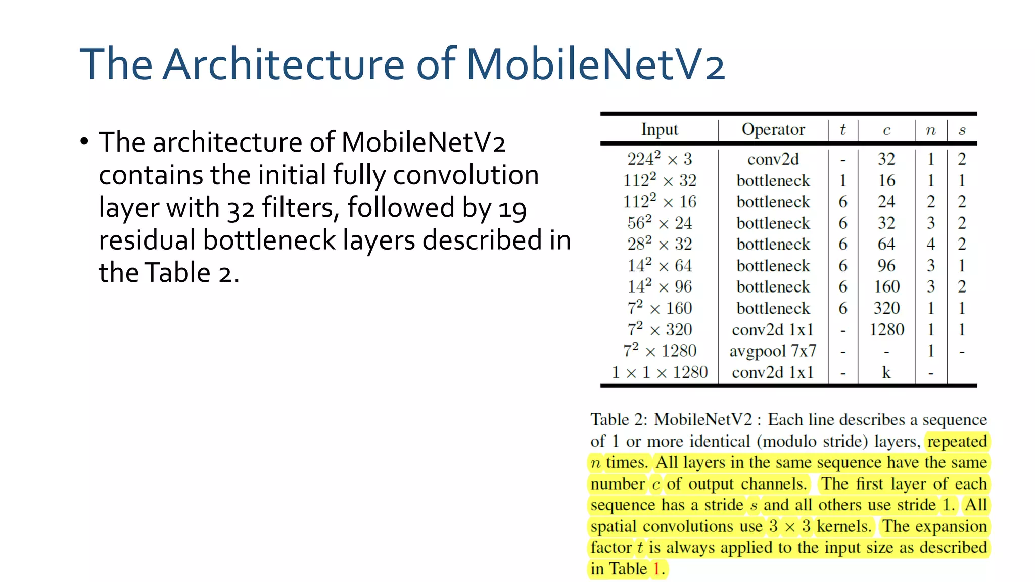
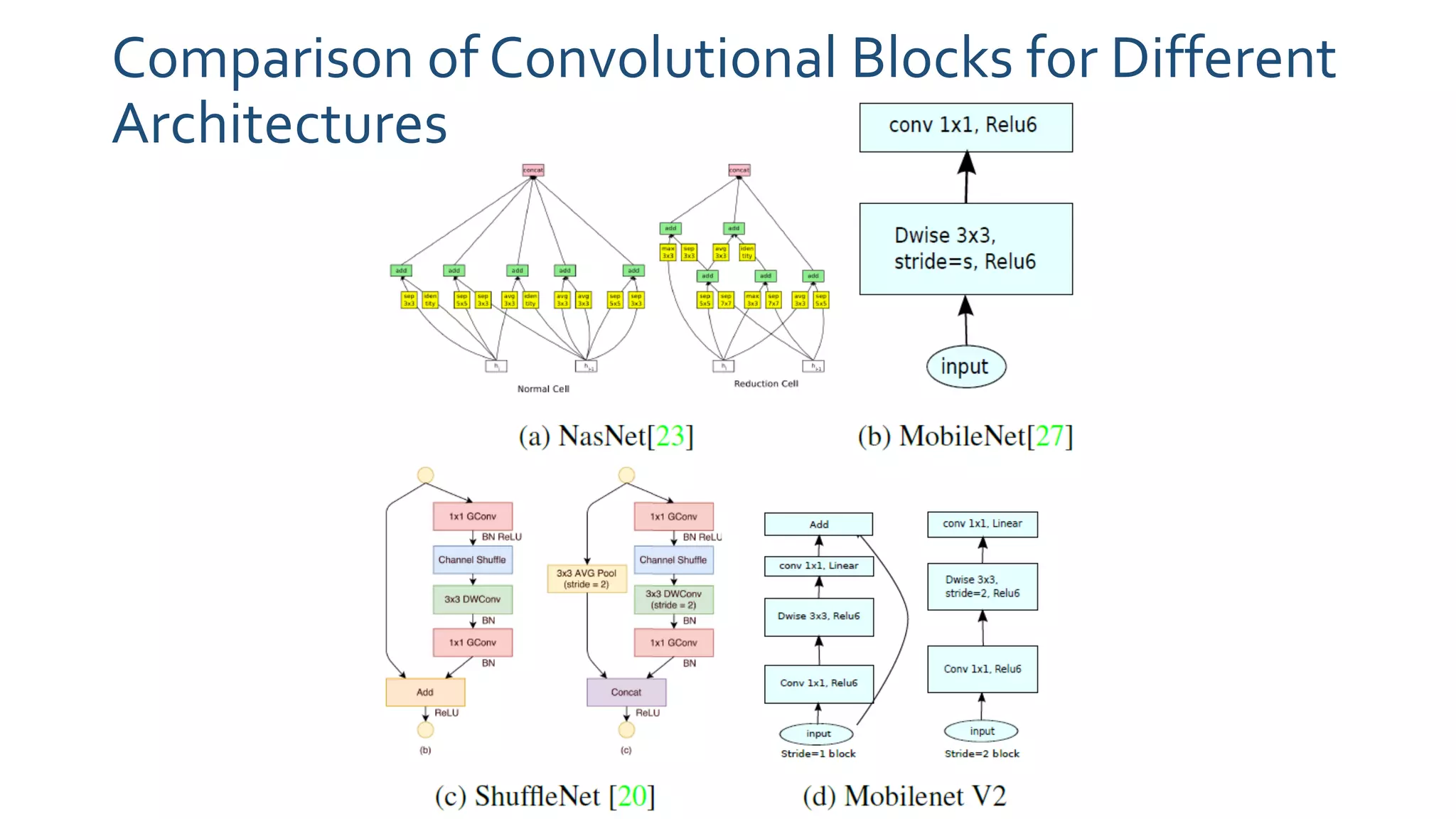
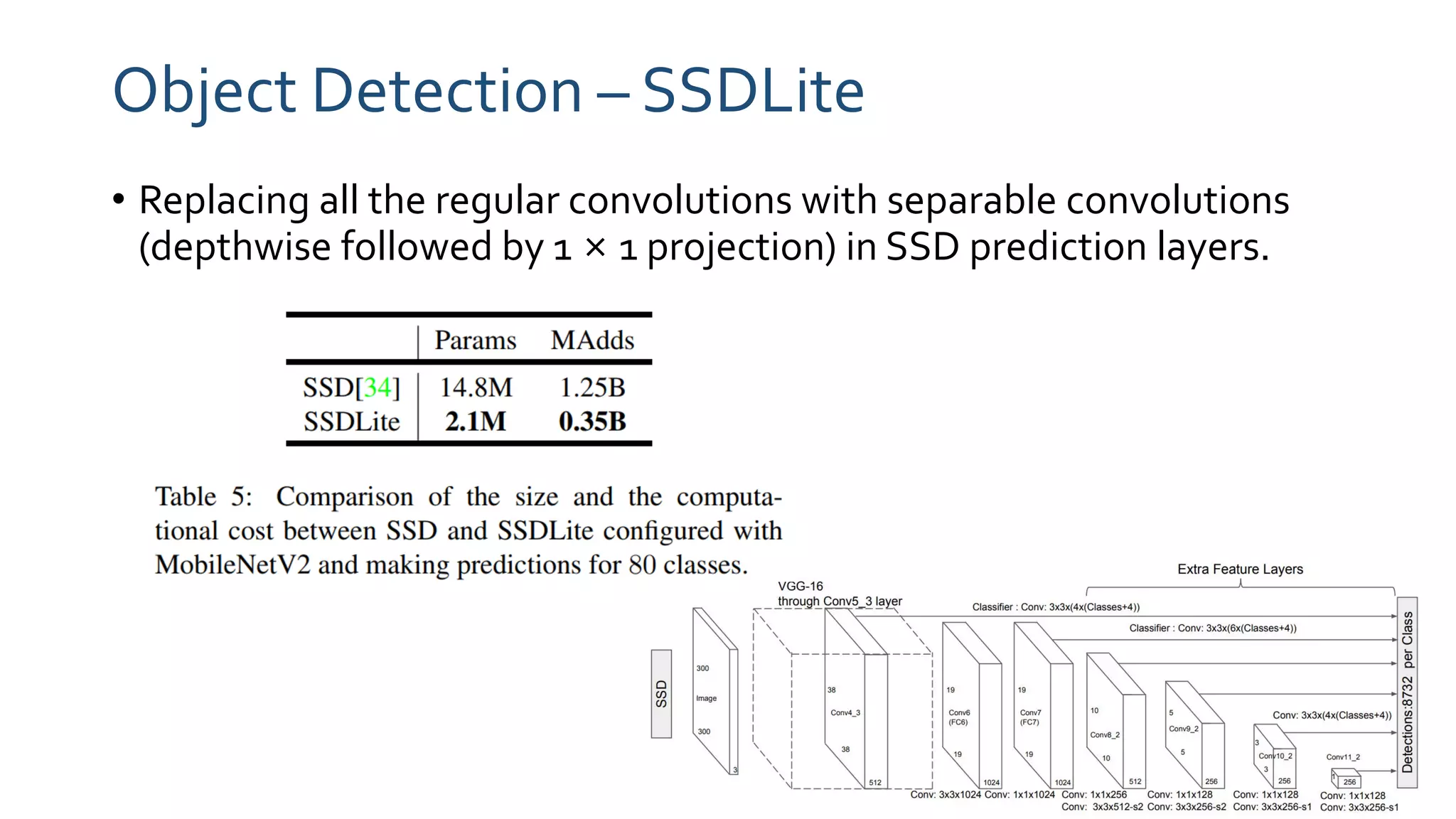
MobileNetV2:
Inverted Residuals and Linear Bottlenecks
7th October, 2018
PR12 Paper Review
Jinwon Lee
Samsung Electronics
Mark Sandler, et al., “MobileNetV2: Inverted Residuals and Linear
Bottlenecks”, CVPR 2018
Related Papers in PR12
• Andrew G. Howard, et al., ” MobileNets: Efficient Convolutional
Neural Networks for MobileVision Applications”
 PR-044 : https://youtu.be/7UoOFKcyIvM
• Xiangyu Zhang, et al., “ShuffleNet: An Extremely Efficient
Convolutional Neural Network for Mobile Devices”
 PR-056 : https://youtu.be/pNuBdj53Hbc
Introduction & RelatedWork
• Modern state of the art networks require high computational
resources beyond the capabilities of many mobile and embedded
applications
• Recently opened up a new direction of bringing optimization
methods including genetic algorithms and reinforcement learning to
architectural search. However one drawback is that the resulting
networks end up very complex.
Recap – MobileNetV1
• Depthwise Separable Convolution (depthwise conv + pointwise conv)
Depthwise
convolution
Pointwise
convolution
Depthwise
convolution
Pointwise
convolution
Figures from https://eli.thegreenplace.net/2018/depthwise-separable-convolutions-for-machine-learning/
http://machinethink.net/blog/googles-mobile-net-architecture-on-iphone/
Recap – MobileNetV1
• Standard convolution takes an ℎ𝑖 × 𝑤𝑖 × 𝑑𝑖 input tensor 𝐿𝑖, and
applies convolutional kernel 𝐾 ∈ 𝑅 𝑘×𝑘×𝑑 𝑖×𝑑 𝑗 to produce an ℎ𝑖 ×
𝑤𝑖 × 𝑑𝑗 output tensor 𝐿𝑗 .
• Standard convolutions have the computational cost of
 ℎ𝑖 × 𝑤𝑖 × 𝑑𝑗 × 𝑘 × 𝑘 × 𝑑𝑖
• Depthwise separable convolutions cost
 ℎ𝑖 × 𝑤𝑖 × 𝑑𝑖 × (𝑘2 + 𝑑𝑗)
• Reduction in computations
 ൗ1
𝑑 𝑗
+ Τ1
𝑘2
 If we use 3x3 depthwise separable convolutions, we get between 8 to 9 times
less computations
Recap – MobileNetV1
Recap – MobileNetV1
• Width Multiplier & Resolution Multiplier
 For a given layer and width multiplier α, the number of input channels M
becomes αM and the number of output channels N becomes αN – where α
with typical settings of 1, 0.75, 0.5 and 0.25
 The second hyper-parameter to reduce the computational cost of a neural
network is a resolution multiplier ρ
Key Features
• Depthwise Separable Convolutions
• Linear Bottlenecks
• Inverted Residuals
Linear Bottlenecks
• Informally, for an input set of real images, we say that the set of layer
activations forms a “manifold of interest”
• It has been long assumed that manifolds of interest in neural
networks could be embedded in low-dimensional subspaces
Linear Bottlenecks
• The authors have highlighted two properties that are indicative of
the requirement that the manifold of interest should lie in a low-
dimensional subspace of the higher-dimensional activation space
1. If the manifold of interest remains non-zero volume after ReLU
transformation, it corresponds to a linear transformation.
2. ReLU is capable of preserving complete information about the input
manifold, but only if the input manifold lies in a low-dimensional subspace
of the input space.
• Assuming the manifold of interest is low-dimensional we can capture
this by inserting linear bottleneck layers into the convolutional blocks
Residual Blocks
• Residual blocks connect the beginning and end of a convolutional
block with a shortcut connection. By adding these two states the
network has the opportunity of accessing earlier activations that
weren’t modified in the convolutional block.
• wide  narrow(bottleneck)  wide approach
Inverted Residuals
• Inspired by the intuition that the bottlenecks actually contain all the
necessary information, while an expansion layer acts merely as an
implementation detail that accompanies a non-linear transformation
of the tensor, the authors use shortcuts directly between the
bottlenecks
• narrow  wide  narrow approach
Bottleneck Residual Blocks
• The basic building block is a bottleneck depth-separable convolution
with residuals
Figures from http://machinethink.net/blog/mobilenet-v2/
# of Operations
• For a block of size ℎ × 𝑤, expansion factor 𝑡 and kernel size 𝑘 with 𝑑′
input channels and 𝑑′′ output channels,
• The total number of multiply add required is
ℎ × 𝑤 × 𝑡 × 𝑑′
× 𝑑′
+ ℎ × 𝑤 × 𝑡 × 𝑑′
× 𝑘 × 𝑘 × 𝑑′
+ ℎ × 𝑤 × 𝑑′′ × 𝑡 × 𝑑′
= ℎ ∙ 𝑤 ∙ 𝑑′ ∙ 𝑡(𝑑′ + 𝑘2 + 𝑑′′)
Information Flow Interpretation
• The proposed convolutional block has a unique property that allows
to separate the network expressiveness (encoded by expansion
layers) from its capacity (encoded by bottleneck inputs).
Figures from http://machinethink.net/blog/mobilenet-v2/
The Architecture of MobileNetV2
• The architecture of MobileNetV2
contains the initial fully convolution
layer with 32 filters, followed by 19
residual bottleneck layers described in
theTable 2.
Trade-off Hyper Parameters
• Input Resolution
 From 96 to 224
• Width Multiplier
 From 0.35 to 1.4
Memory Efficient Inference
• The amount of memory is simply the maximum total size of
combined inputs and outputs across all operations.
• If we treat a bottleneck residual block as a single operation (and treat
inner convolution as a disposable tensor), the total amount of
memory would be dominated by the size of bottleneck tensors,
rather than the size of tensors that are internal to bottleneck (and
much larger)
Bottleneck Residual Block – ATrick for Reducing
Memory Requirement
• A bottleneck block operator 𝐹(𝑥) can be expressed as a composition of
three operators 𝐹 𝑥 = 𝐴 ∘ 𝑁 ∘ 𝐵 𝑥
• 𝐴, 𝐵 is a linear transform, 𝑁 = 𝑅𝑒𝐿𝑈6 ∘ 𝑑𝑤𝑖𝑠𝑒 ∘ 𝑅𝑒𝐿𝑈6
• 𝐴: 𝑅 𝑠×𝑠×𝑘 → 𝑅 𝑠×𝑠×𝑛, 𝑁: 𝑅 𝑠×𝑠×𝑛 → 𝑅 𝑠′×𝑠′×𝑛, 𝐵: 𝑅 𝑠′×𝑠′×𝑘 → 𝑅 𝑠′×𝑠′×𝑛
• The algorithm is based on the fact that the inner tensor 𝐼 can be
represented as concatenation of 𝑡 tensors, of size 𝑛/𝑡 each and our
function can then be represented as 𝐹 𝑥 = σ𝑖=1
𝑡
(𝐴𝑖 ∘ 𝑁 ∘ 𝐵𝑖)(𝑥)
• Using 𝑛 = 𝑡 we end up having to keep only a single channel of the
intermediate representation at all times
• The authors find that this approach is the most helpful to be used with 𝑡
being a small constant between 2 and 5
 Too small 𝑡 causes cache misses
Comparison of Convolutional Blocks for Different
Architectures
The Max Number of Channels/Memory(in Kb)
ImageNet Classification Results
Vs MobileNetV1
Data from http://machinethink.net/blog/mobilenet-v2/
Object Detection – SSDLite
• Replacing all the regular convolutions with separable convolutions
(depthwise followed by 1 × 1 projection) in SSD prediction layers.
Object Detection Results
Semantic Segmentation Results
The Impact of Non-linearities andVariousTypes
of Shortcut Connections

PR-108: MobileNetV2: Inverted Residuals and Linear Bottlenecks

  • 1.
    MobileNetV2: Inverted Residuals andLinear Bottlenecks 7th October, 2018 PR12 Paper Review Jinwon Lee Samsung Electronics Mark Sandler, et al., “MobileNetV2: Inverted Residuals and Linear Bottlenecks”, CVPR 2018
  • 2.
    Related Papers inPR12 • Andrew G. Howard, et al., ” MobileNets: Efficient Convolutional Neural Networks for MobileVision Applications”  PR-044 : https://youtu.be/7UoOFKcyIvM • Xiangyu Zhang, et al., “ShuffleNet: An Extremely Efficient Convolutional Neural Network for Mobile Devices”  PR-056 : https://youtu.be/pNuBdj53Hbc
  • 3.
    Introduction & RelatedWork •Modern state of the art networks require high computational resources beyond the capabilities of many mobile and embedded applications • Recently opened up a new direction of bringing optimization methods including genetic algorithms and reinforcement learning to architectural search. However one drawback is that the resulting networks end up very complex.
  • 4.
    Recap – MobileNetV1 •Depthwise Separable Convolution (depthwise conv + pointwise conv) Depthwise convolution Pointwise convolution Depthwise convolution Pointwise convolution Figures from https://eli.thegreenplace.net/2018/depthwise-separable-convolutions-for-machine-learning/ http://machinethink.net/blog/googles-mobile-net-architecture-on-iphone/
  • 5.
    Recap – MobileNetV1 •Standard convolution takes an ℎ𝑖 × 𝑤𝑖 × 𝑑𝑖 input tensor 𝐿𝑖, and applies convolutional kernel 𝐾 ∈ 𝑅 𝑘×𝑘×𝑑 𝑖×𝑑 𝑗 to produce an ℎ𝑖 × 𝑤𝑖 × 𝑑𝑗 output tensor 𝐿𝑗 . • Standard convolutions have the computational cost of  ℎ𝑖 × 𝑤𝑖 × 𝑑𝑗 × 𝑘 × 𝑘 × 𝑑𝑖 • Depthwise separable convolutions cost  ℎ𝑖 × 𝑤𝑖 × 𝑑𝑖 × (𝑘2 + 𝑑𝑗) • Reduction in computations  ൗ1 𝑑 𝑗 + Τ1 𝑘2  If we use 3x3 depthwise separable convolutions, we get between 8 to 9 times less computations
  • 6.
  • 7.
    Recap – MobileNetV1 •Width Multiplier & Resolution Multiplier  For a given layer and width multiplier α, the number of input channels M becomes αM and the number of output channels N becomes αN – where α with typical settings of 1, 0.75, 0.5 and 0.25  The second hyper-parameter to reduce the computational cost of a neural network is a resolution multiplier ρ
  • 8.
    Key Features • DepthwiseSeparable Convolutions • Linear Bottlenecks • Inverted Residuals
  • 9.
    Linear Bottlenecks • Informally,for an input set of real images, we say that the set of layer activations forms a “manifold of interest” • It has been long assumed that manifolds of interest in neural networks could be embedded in low-dimensional subspaces
  • 10.
    Linear Bottlenecks • Theauthors have highlighted two properties that are indicative of the requirement that the manifold of interest should lie in a low- dimensional subspace of the higher-dimensional activation space 1. If the manifold of interest remains non-zero volume after ReLU transformation, it corresponds to a linear transformation. 2. ReLU is capable of preserving complete information about the input manifold, but only if the input manifold lies in a low-dimensional subspace of the input space. • Assuming the manifold of interest is low-dimensional we can capture this by inserting linear bottleneck layers into the convolutional blocks
  • 11.
    Residual Blocks • Residualblocks connect the beginning and end of a convolutional block with a shortcut connection. By adding these two states the network has the opportunity of accessing earlier activations that weren’t modified in the convolutional block. • wide  narrow(bottleneck)  wide approach
  • 12.
    Inverted Residuals • Inspiredby the intuition that the bottlenecks actually contain all the necessary information, while an expansion layer acts merely as an implementation detail that accompanies a non-linear transformation of the tensor, the authors use shortcuts directly between the bottlenecks • narrow  wide  narrow approach
  • 13.
    Bottleneck Residual Blocks •The basic building block is a bottleneck depth-separable convolution with residuals Figures from http://machinethink.net/blog/mobilenet-v2/
  • 14.
    # of Operations •For a block of size ℎ × 𝑤, expansion factor 𝑡 and kernel size 𝑘 with 𝑑′ input channels and 𝑑′′ output channels, • The total number of multiply add required is ℎ × 𝑤 × 𝑡 × 𝑑′ × 𝑑′ + ℎ × 𝑤 × 𝑡 × 𝑑′ × 𝑘 × 𝑘 × 𝑑′ + ℎ × 𝑤 × 𝑑′′ × 𝑡 × 𝑑′ = ℎ ∙ 𝑤 ∙ 𝑑′ ∙ 𝑡(𝑑′ + 𝑘2 + 𝑑′′)
  • 15.
    Information Flow Interpretation •The proposed convolutional block has a unique property that allows to separate the network expressiveness (encoded by expansion layers) from its capacity (encoded by bottleneck inputs). Figures from http://machinethink.net/blog/mobilenet-v2/
  • 16.
    The Architecture ofMobileNetV2 • The architecture of MobileNetV2 contains the initial fully convolution layer with 32 filters, followed by 19 residual bottleneck layers described in theTable 2.
  • 17.
    Trade-off Hyper Parameters •Input Resolution  From 96 to 224 • Width Multiplier  From 0.35 to 1.4
  • 18.
    Memory Efficient Inference •The amount of memory is simply the maximum total size of combined inputs and outputs across all operations. • If we treat a bottleneck residual block as a single operation (and treat inner convolution as a disposable tensor), the total amount of memory would be dominated by the size of bottleneck tensors, rather than the size of tensors that are internal to bottleneck (and much larger)
  • 19.
    Bottleneck Residual Block– ATrick for Reducing Memory Requirement • A bottleneck block operator 𝐹(𝑥) can be expressed as a composition of three operators 𝐹 𝑥 = 𝐴 ∘ 𝑁 ∘ 𝐵 𝑥 • 𝐴, 𝐵 is a linear transform, 𝑁 = 𝑅𝑒𝐿𝑈6 ∘ 𝑑𝑤𝑖𝑠𝑒 ∘ 𝑅𝑒𝐿𝑈6 • 𝐴: 𝑅 𝑠×𝑠×𝑘 → 𝑅 𝑠×𝑠×𝑛, 𝑁: 𝑅 𝑠×𝑠×𝑛 → 𝑅 𝑠′×𝑠′×𝑛, 𝐵: 𝑅 𝑠′×𝑠′×𝑘 → 𝑅 𝑠′×𝑠′×𝑛 • The algorithm is based on the fact that the inner tensor 𝐼 can be represented as concatenation of 𝑡 tensors, of size 𝑛/𝑡 each and our function can then be represented as 𝐹 𝑥 = σ𝑖=1 𝑡 (𝐴𝑖 ∘ 𝑁 ∘ 𝐵𝑖)(𝑥) • Using 𝑛 = 𝑡 we end up having to keep only a single channel of the intermediate representation at all times • The authors find that this approach is the most helpful to be used with 𝑡 being a small constant between 2 and 5  Too small 𝑡 causes cache misses
  • 20.
    Comparison of ConvolutionalBlocks for Different Architectures
  • 21.
    The Max Numberof Channels/Memory(in Kb)
  • 22.
  • 23.
    Vs MobileNetV1 Data fromhttp://machinethink.net/blog/mobilenet-v2/
  • 24.
    Object Detection –SSDLite • Replacing all the regular convolutions with separable convolutions (depthwise followed by 1 × 1 projection) in SSD prediction layers.
  • 25.
  • 26.
  • 27.
    The Impact ofNon-linearities andVariousTypes of Shortcut Connections