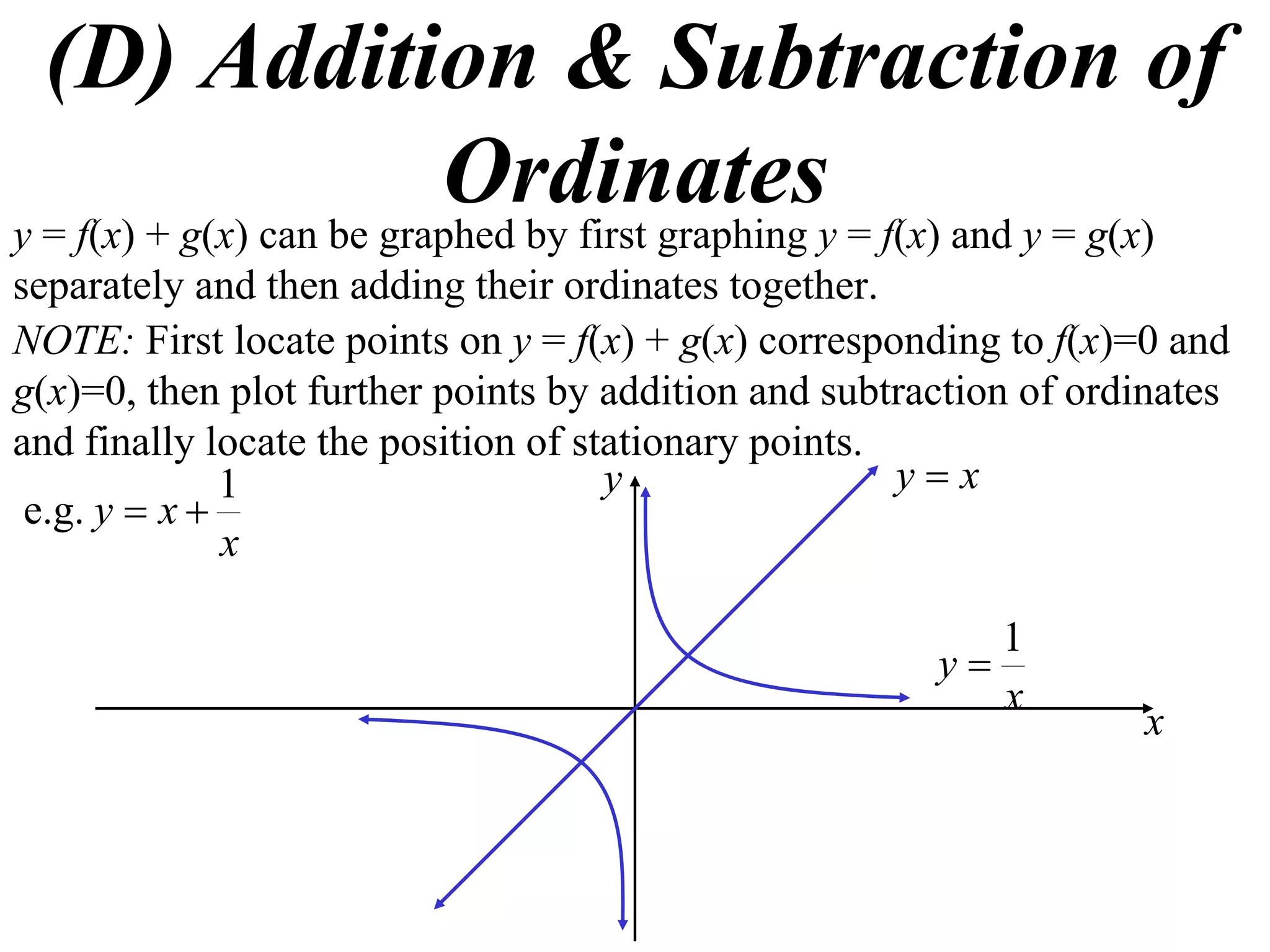
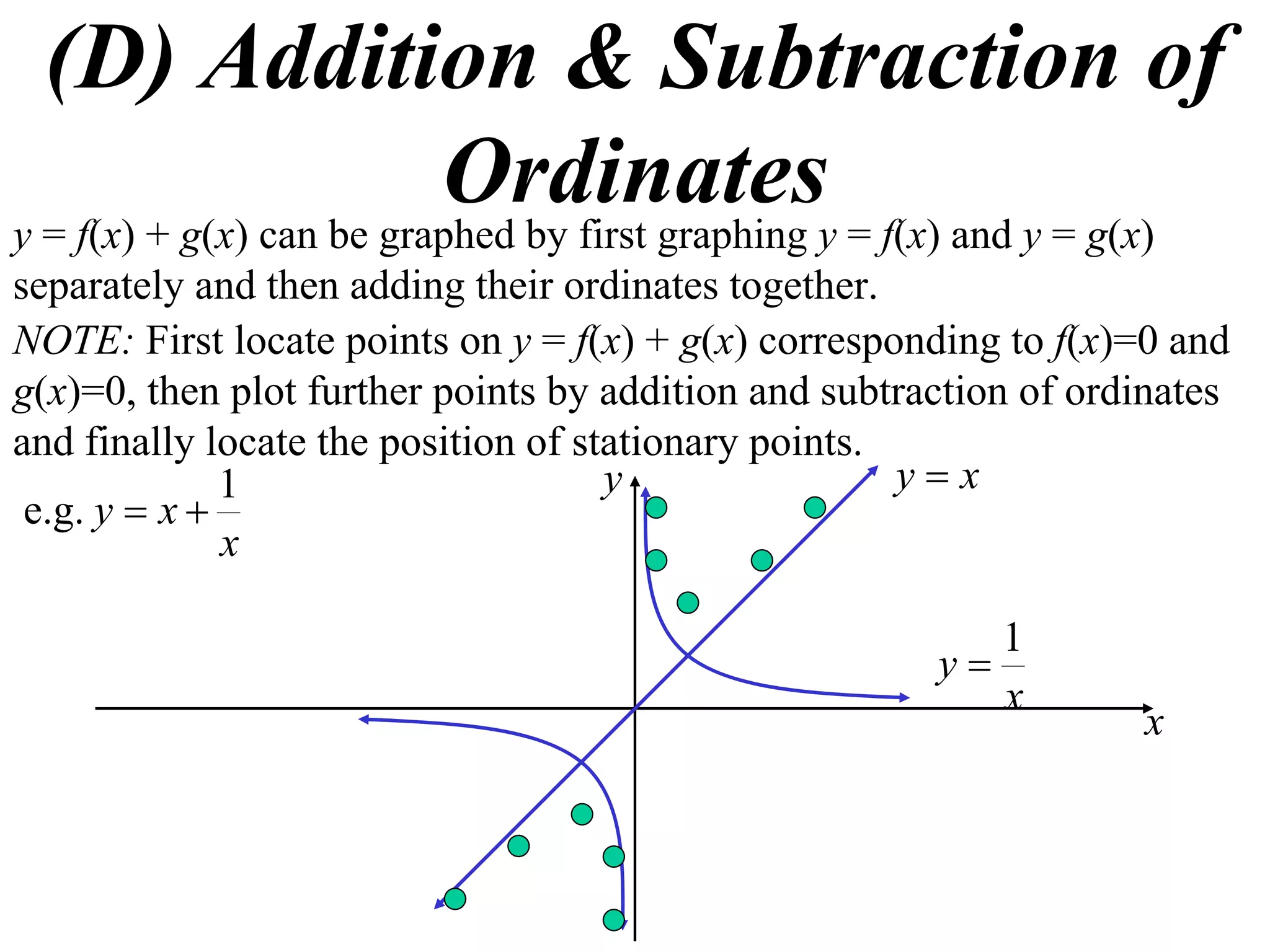
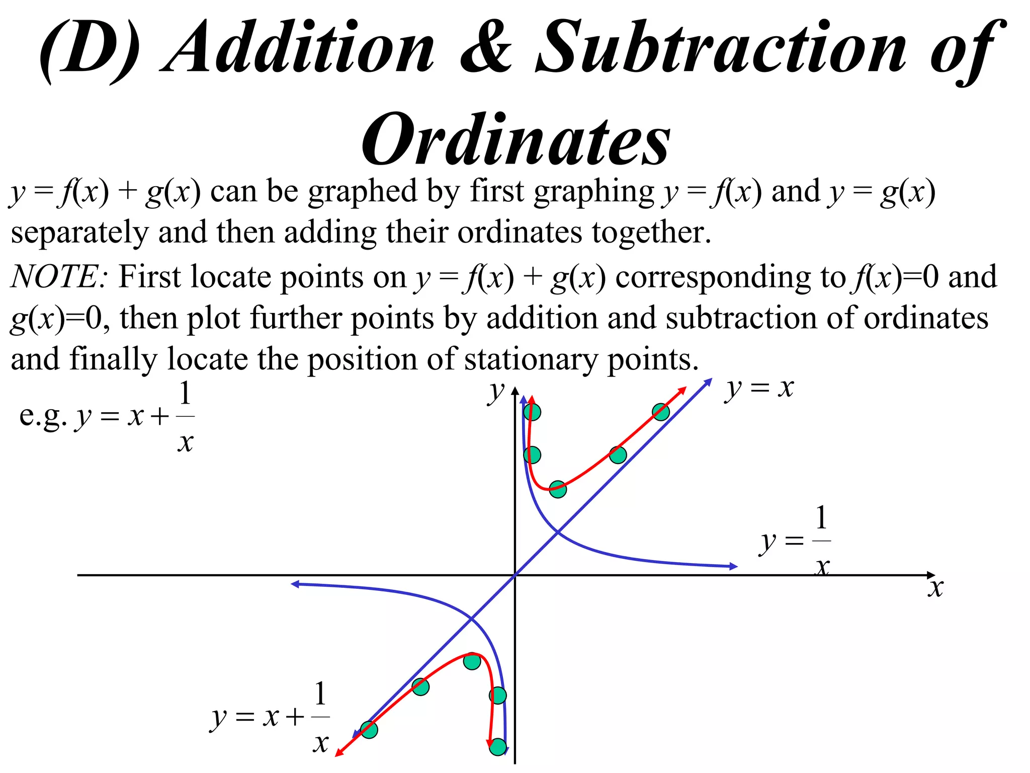
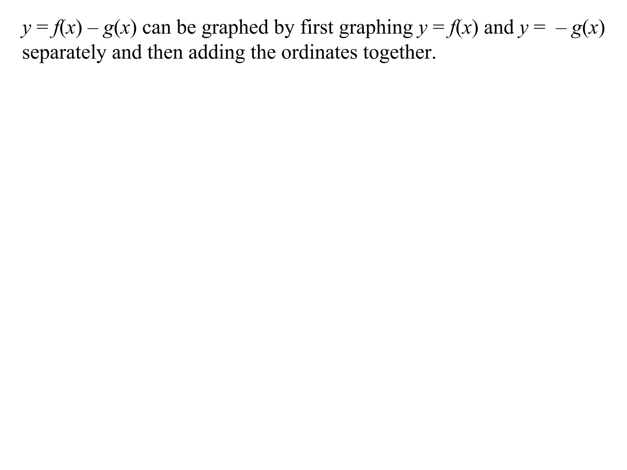
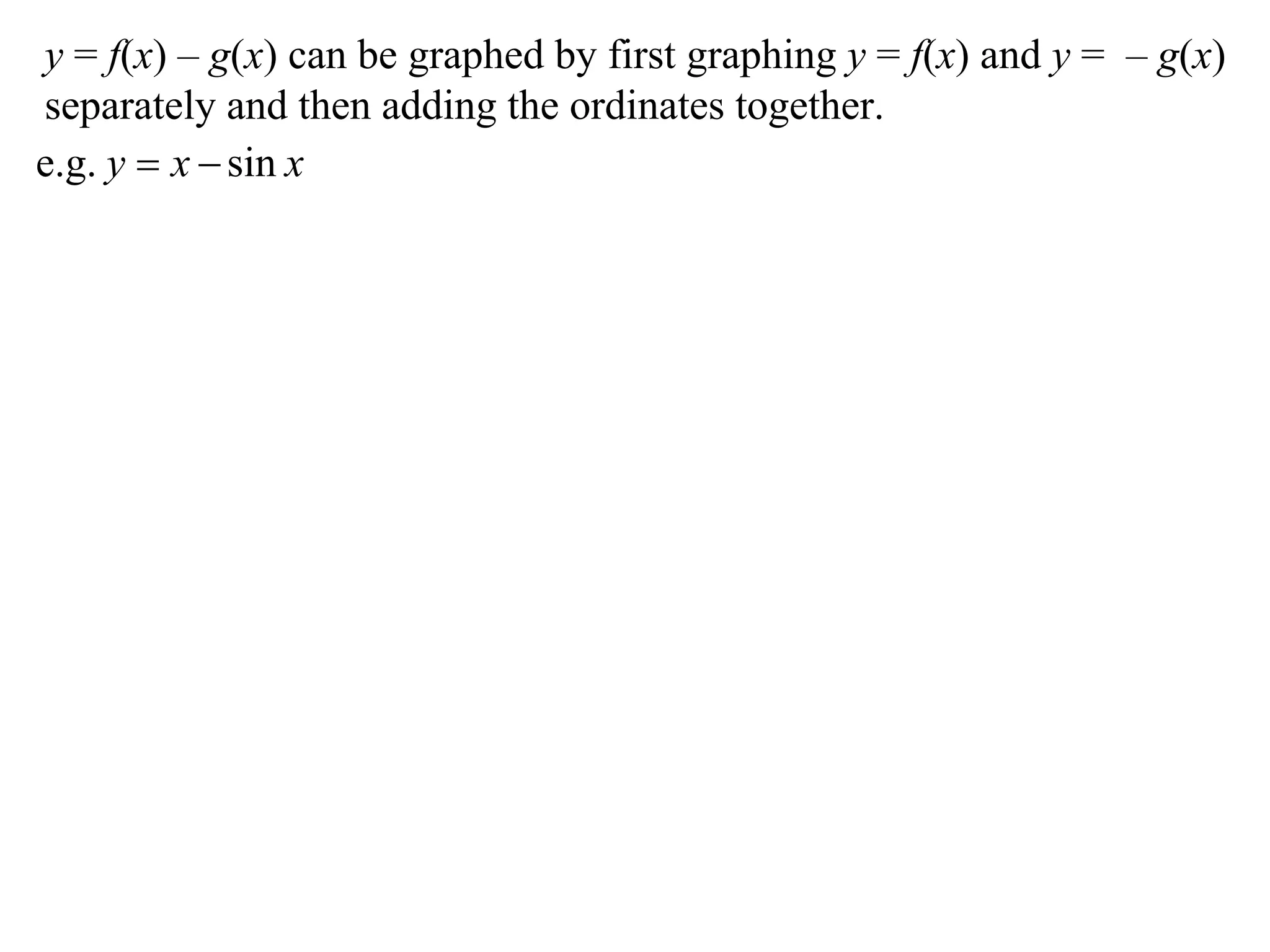
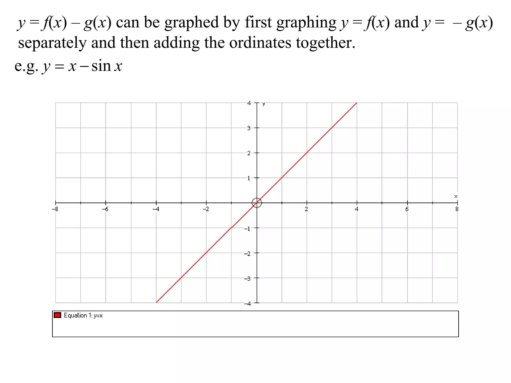
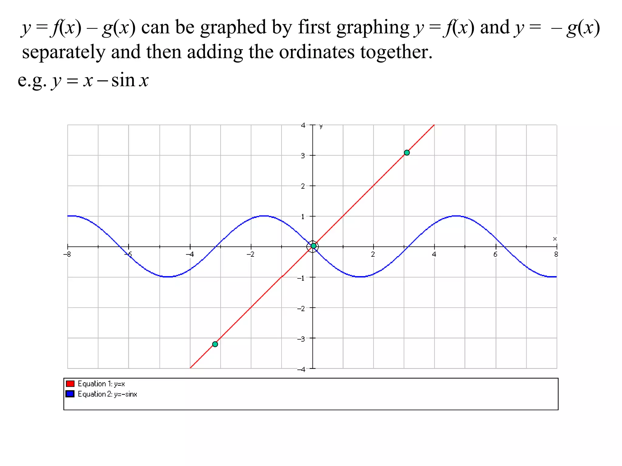
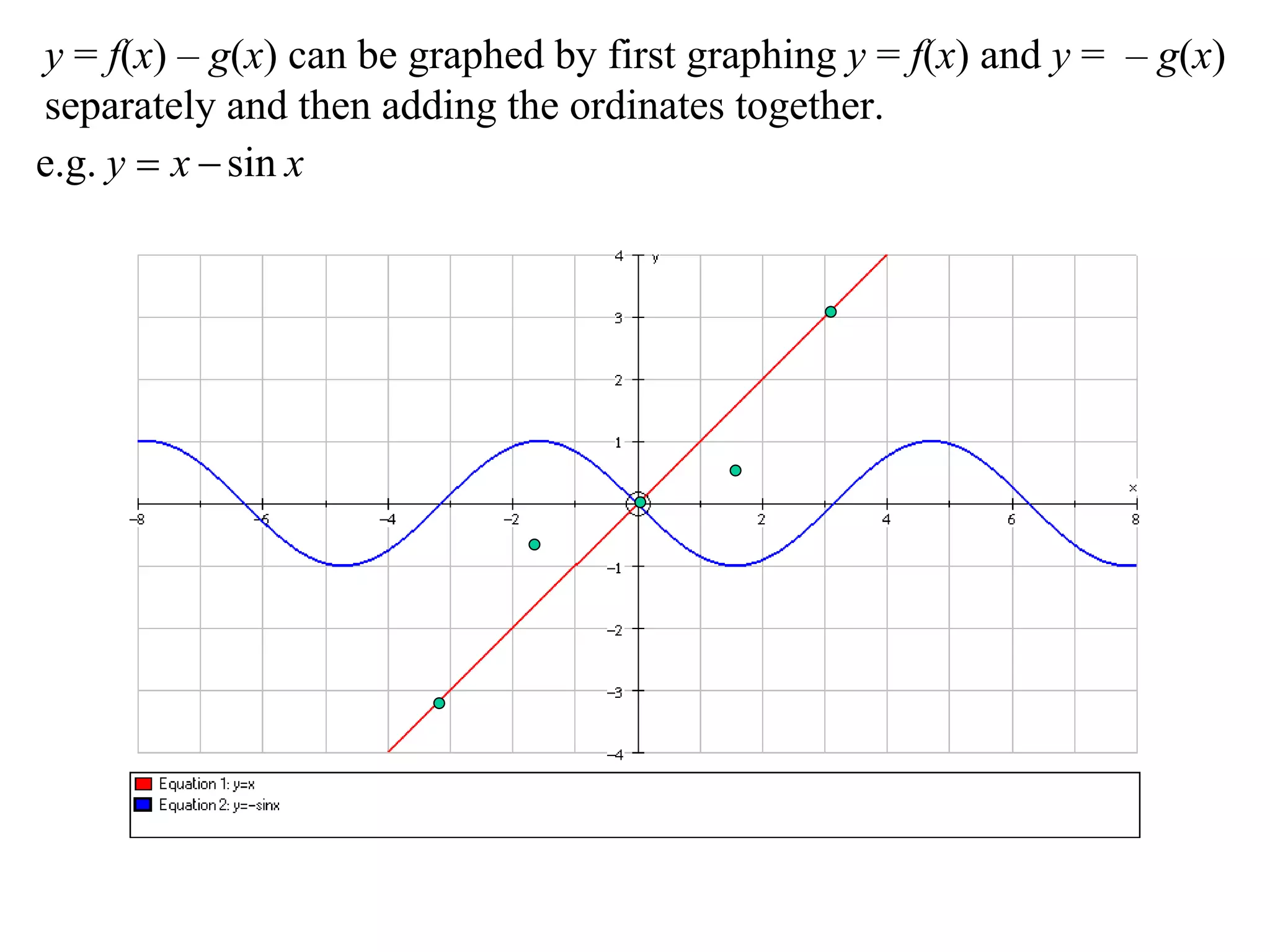
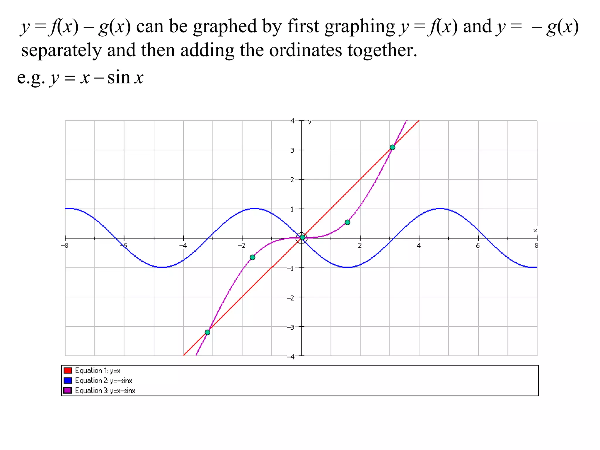
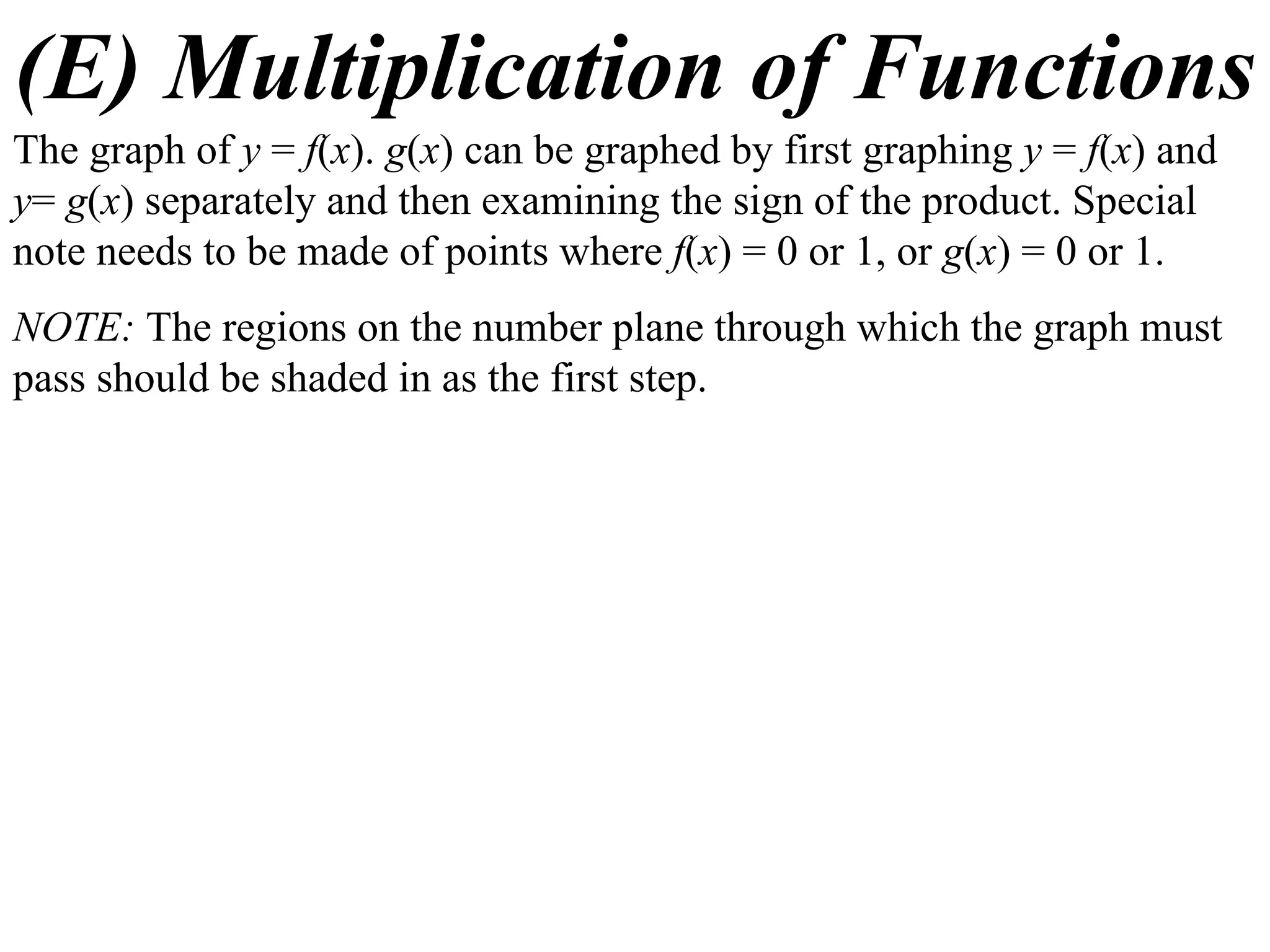
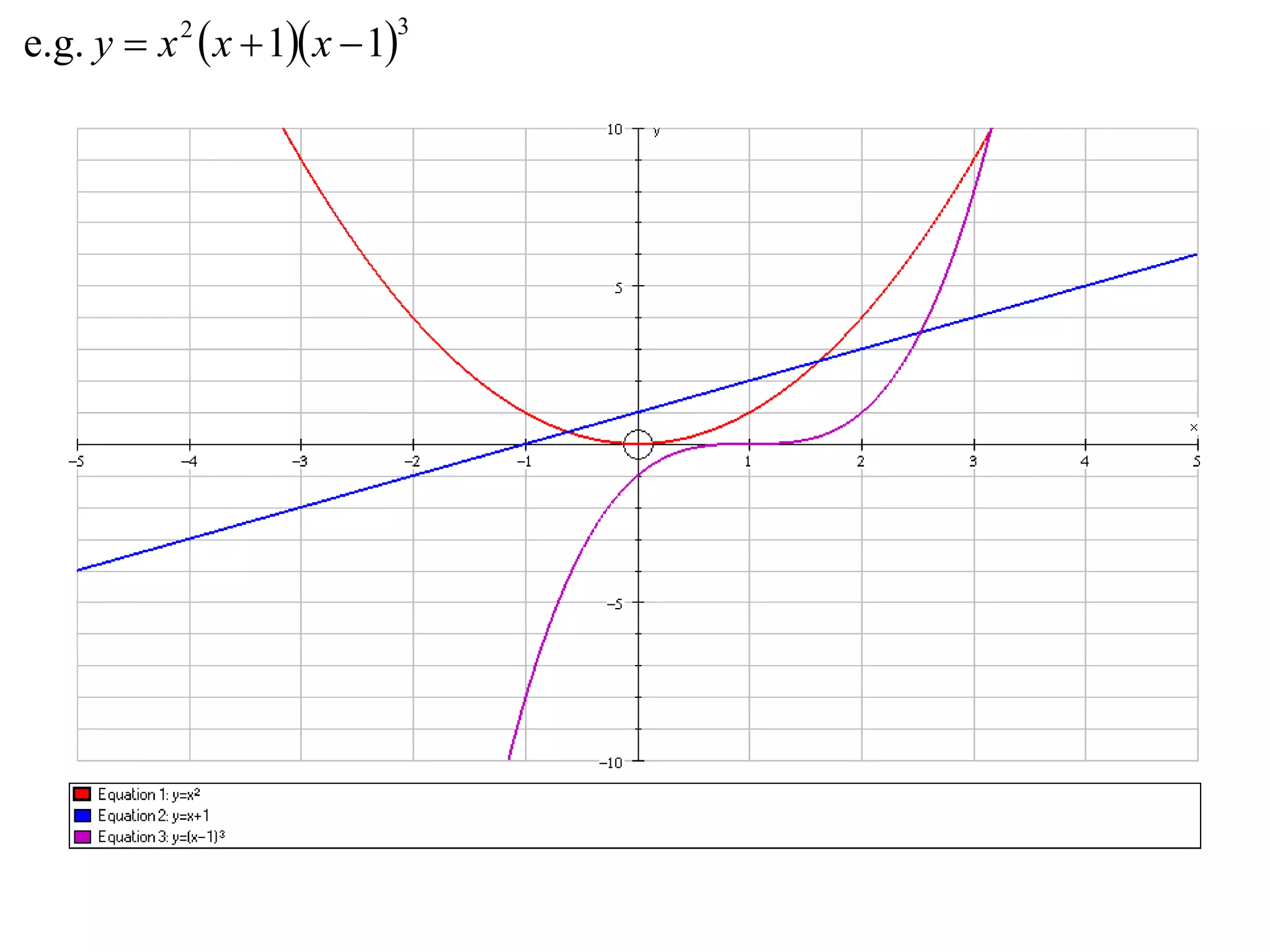
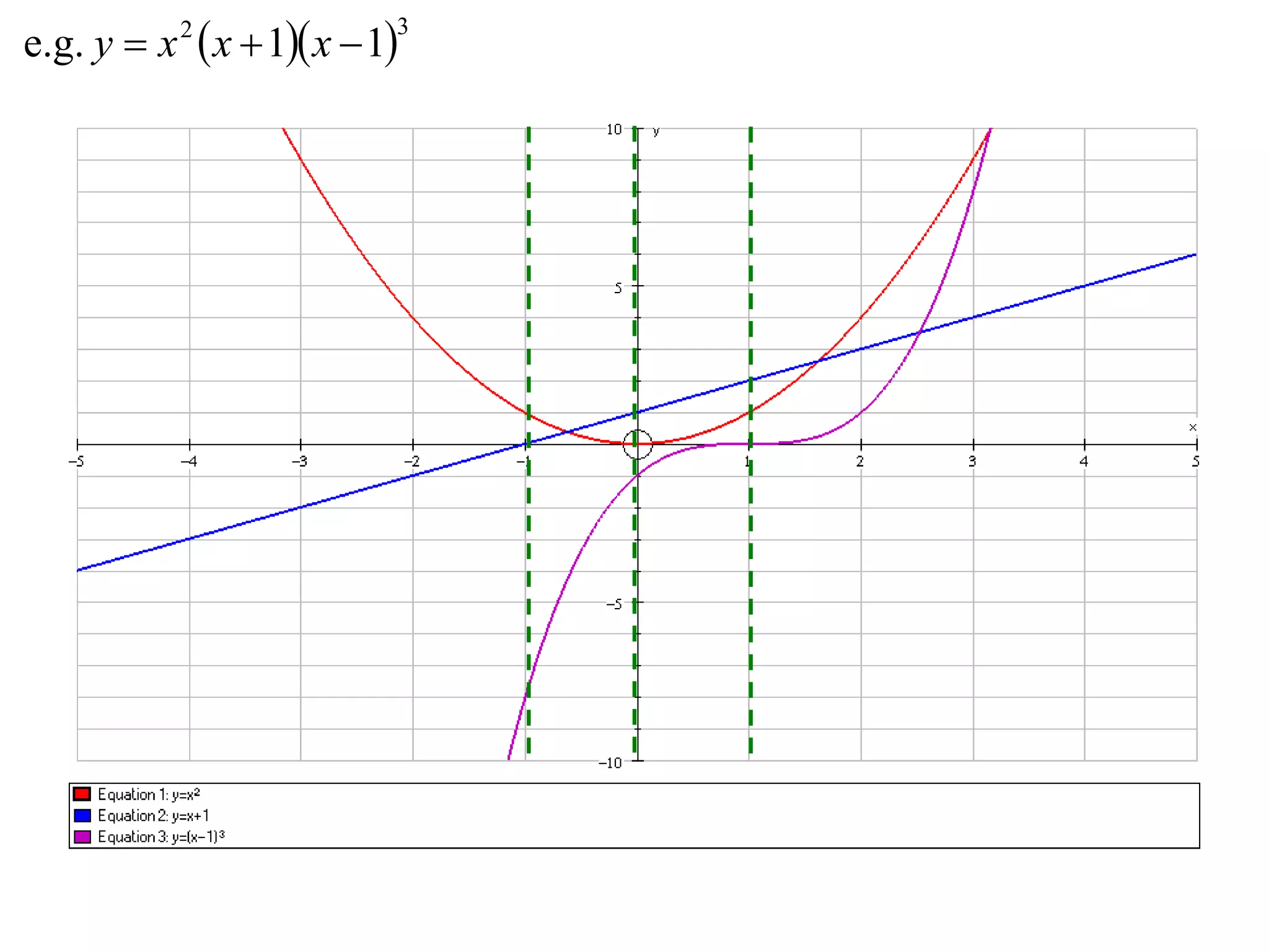
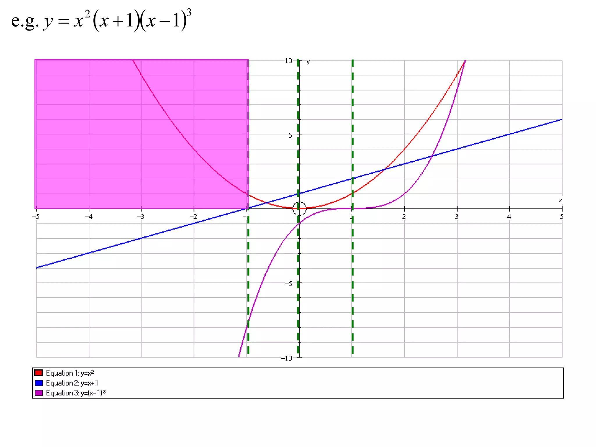
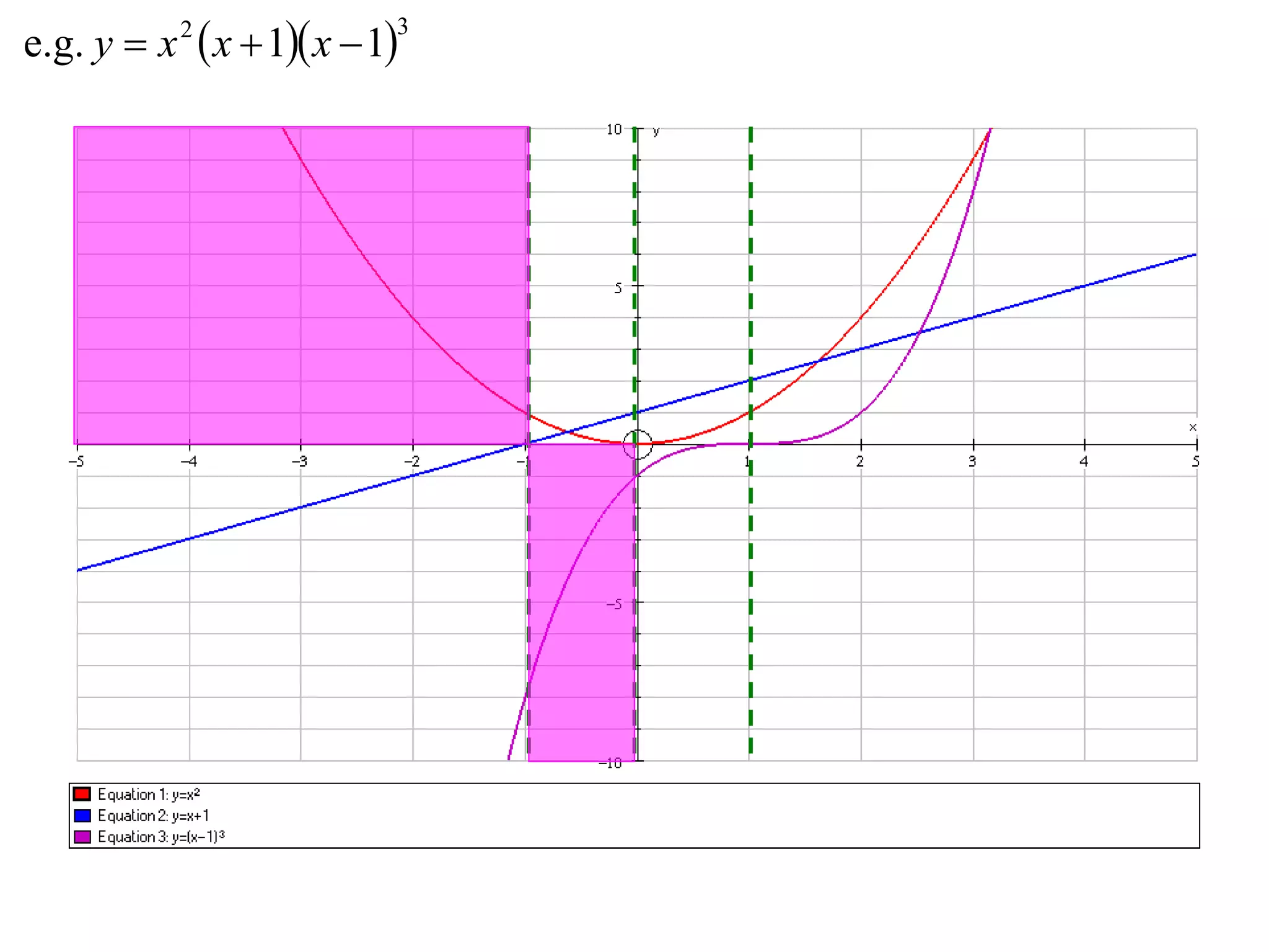
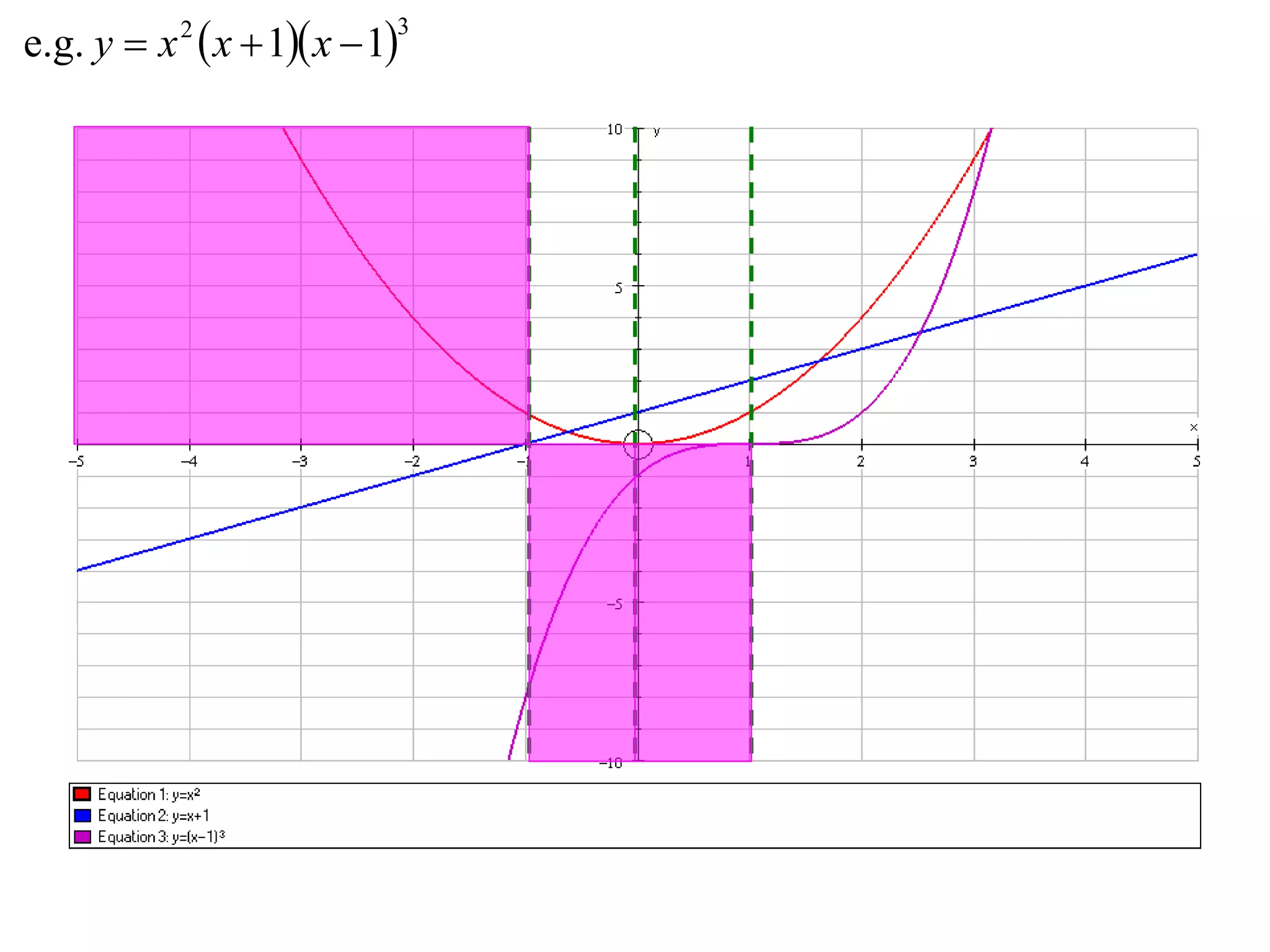
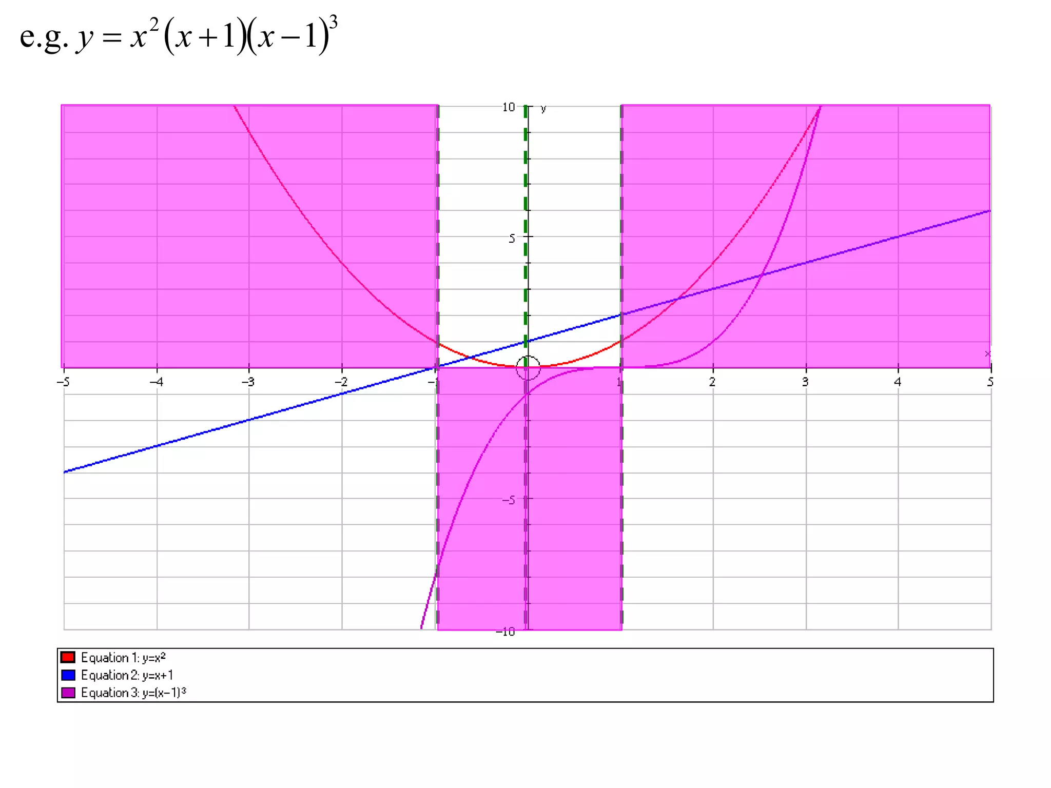
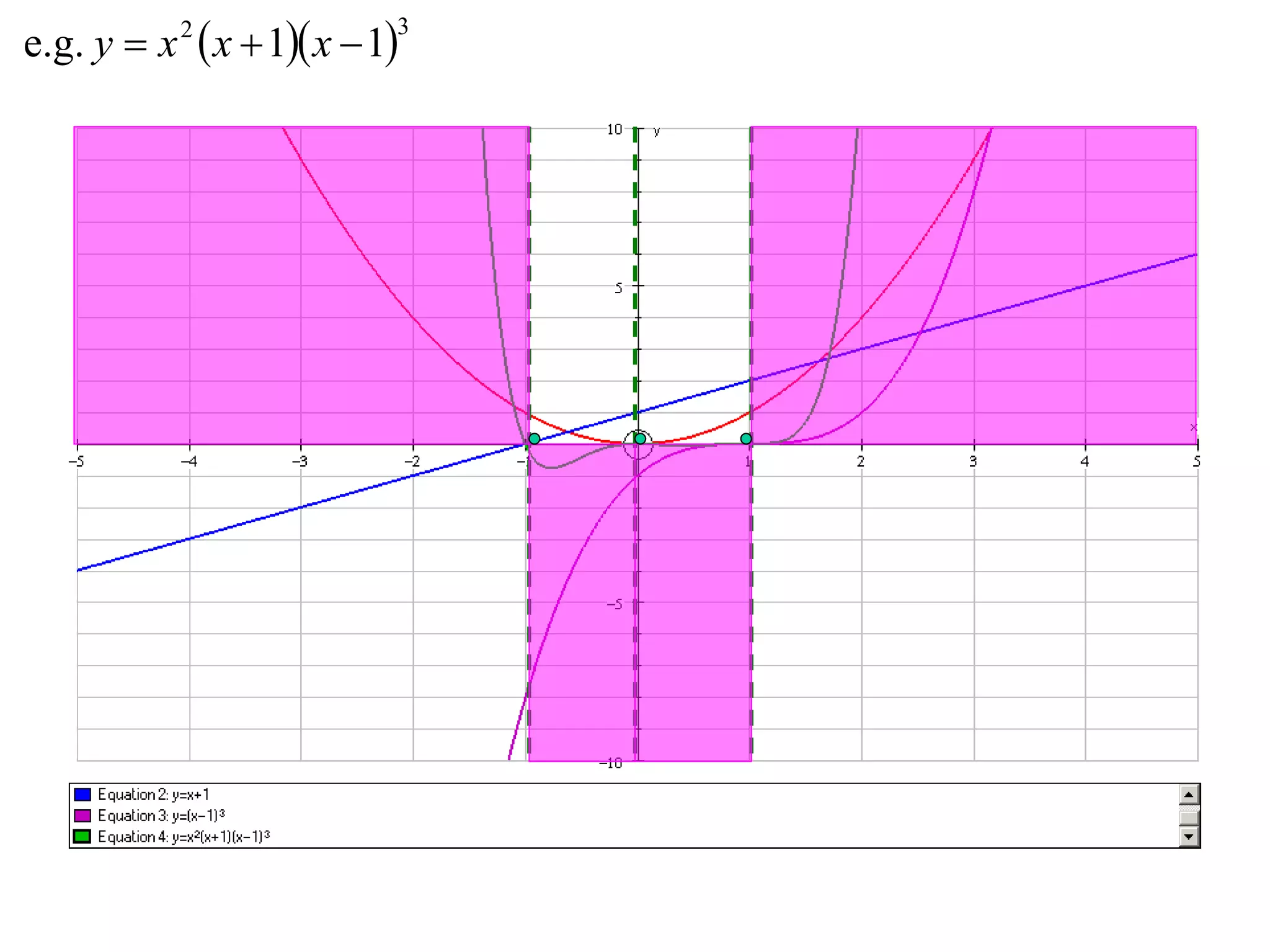
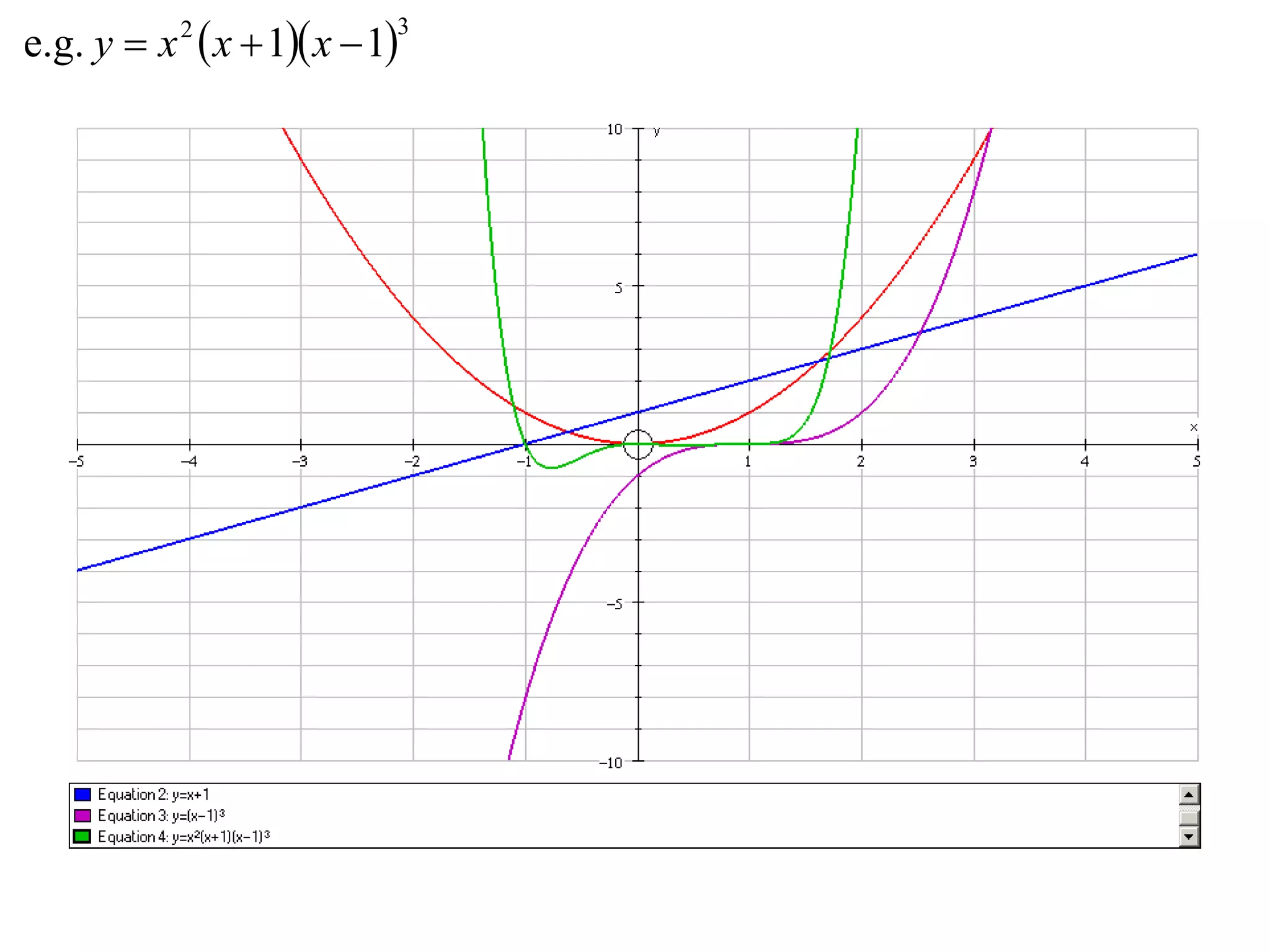
The document describes methods for graphing functions involving addition, subtraction, multiplication, and division of other functions. Specifically: - Addition and subtraction graphs can be made by graphing the added/subtracted functions separately and then combining their ordinates. - Multiplication graphs are made by examining the sign of the product function and noting where factors are 0 or 1. 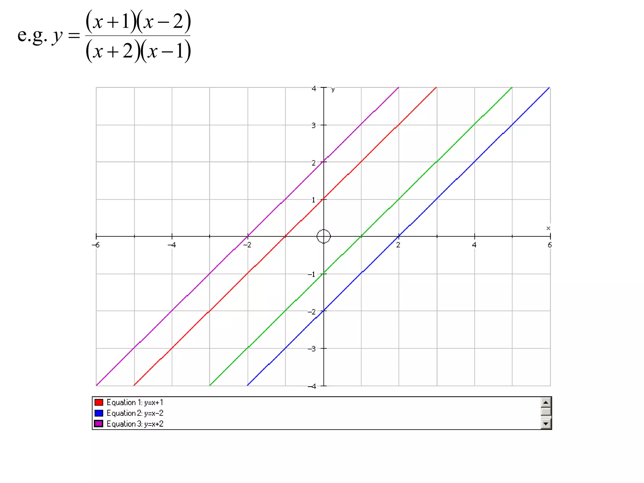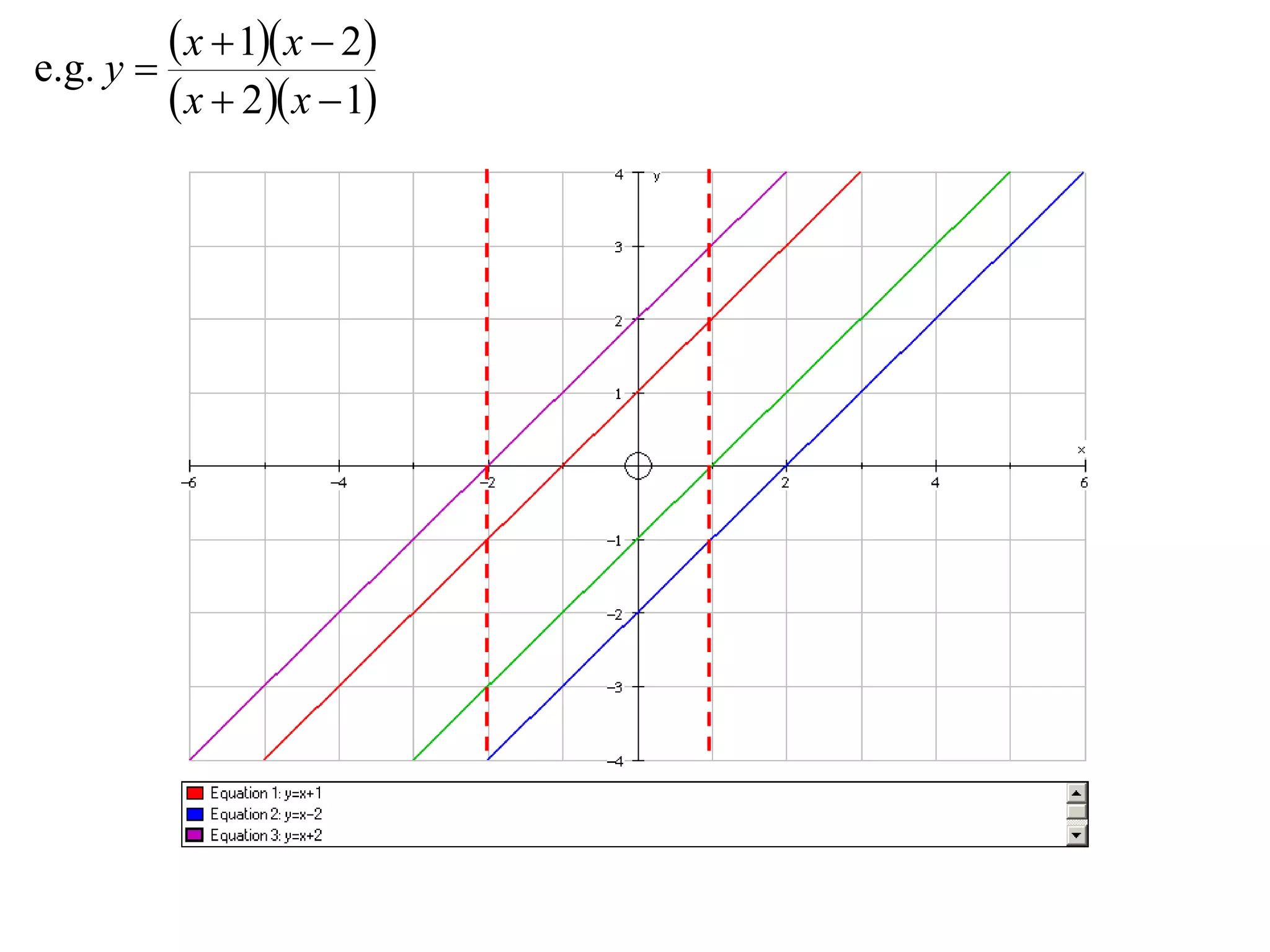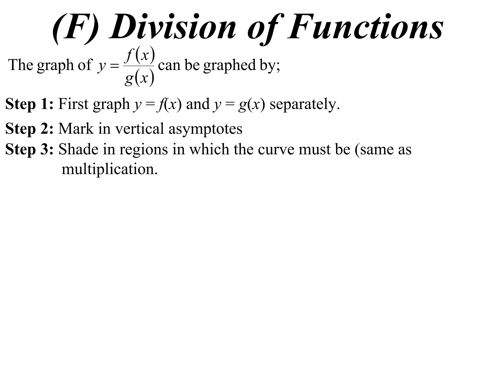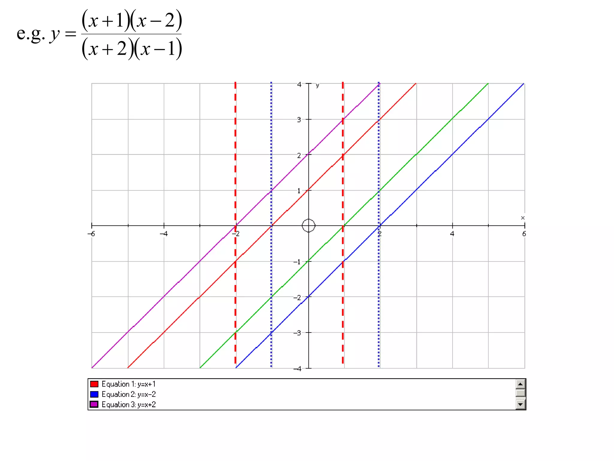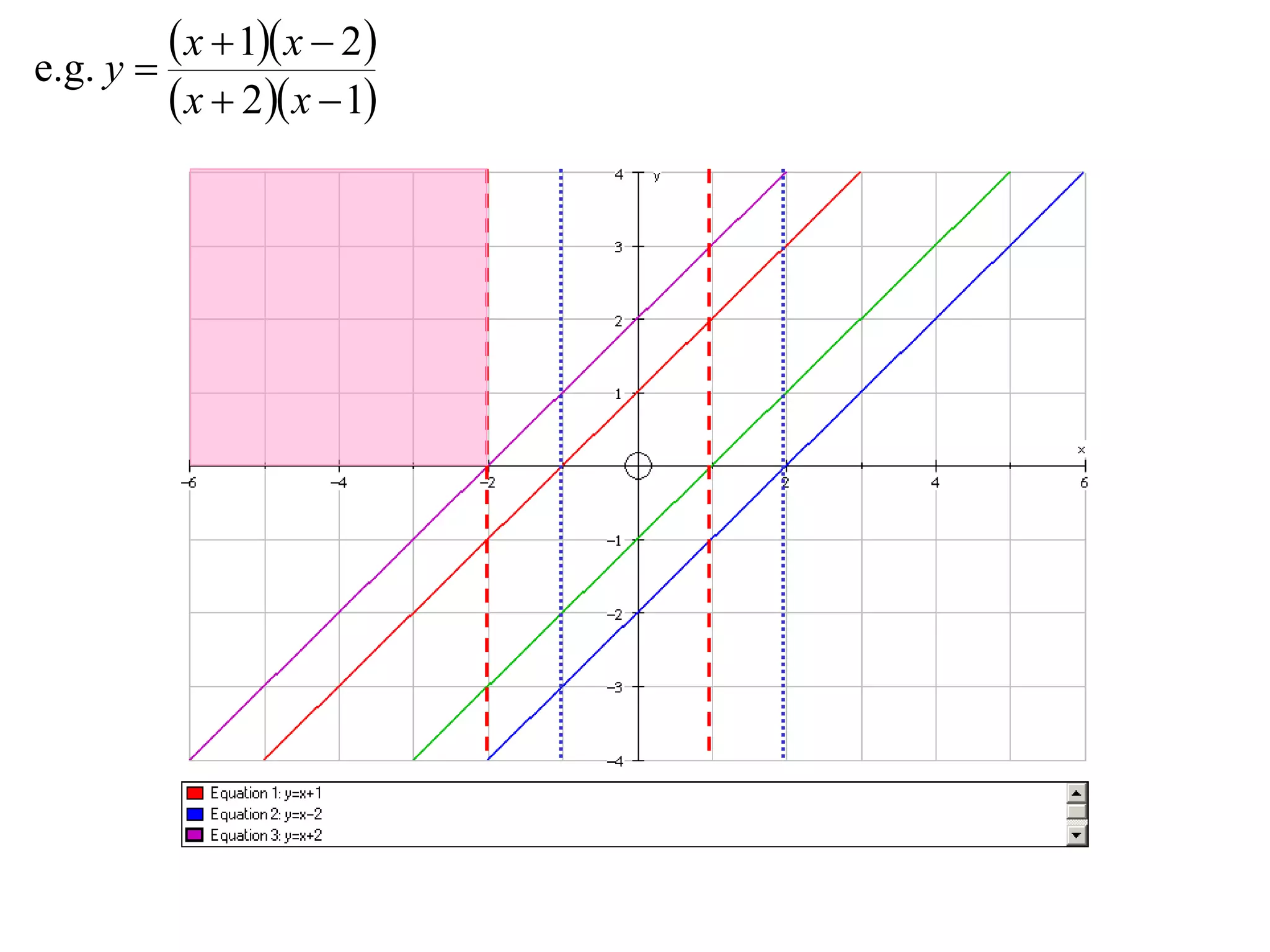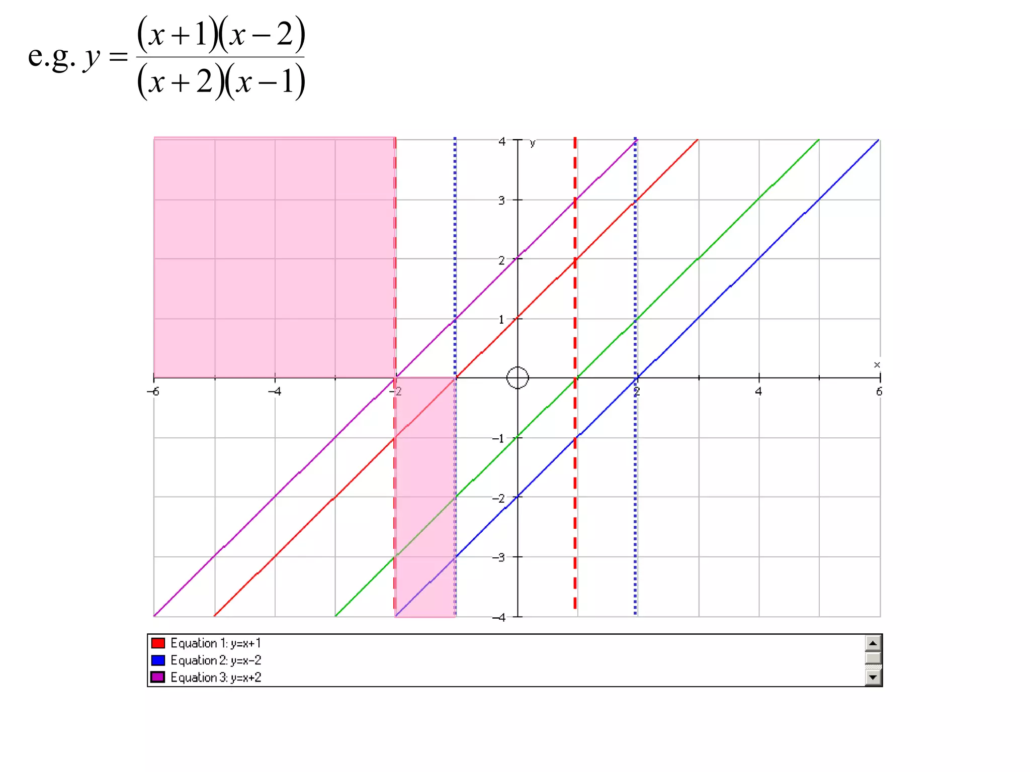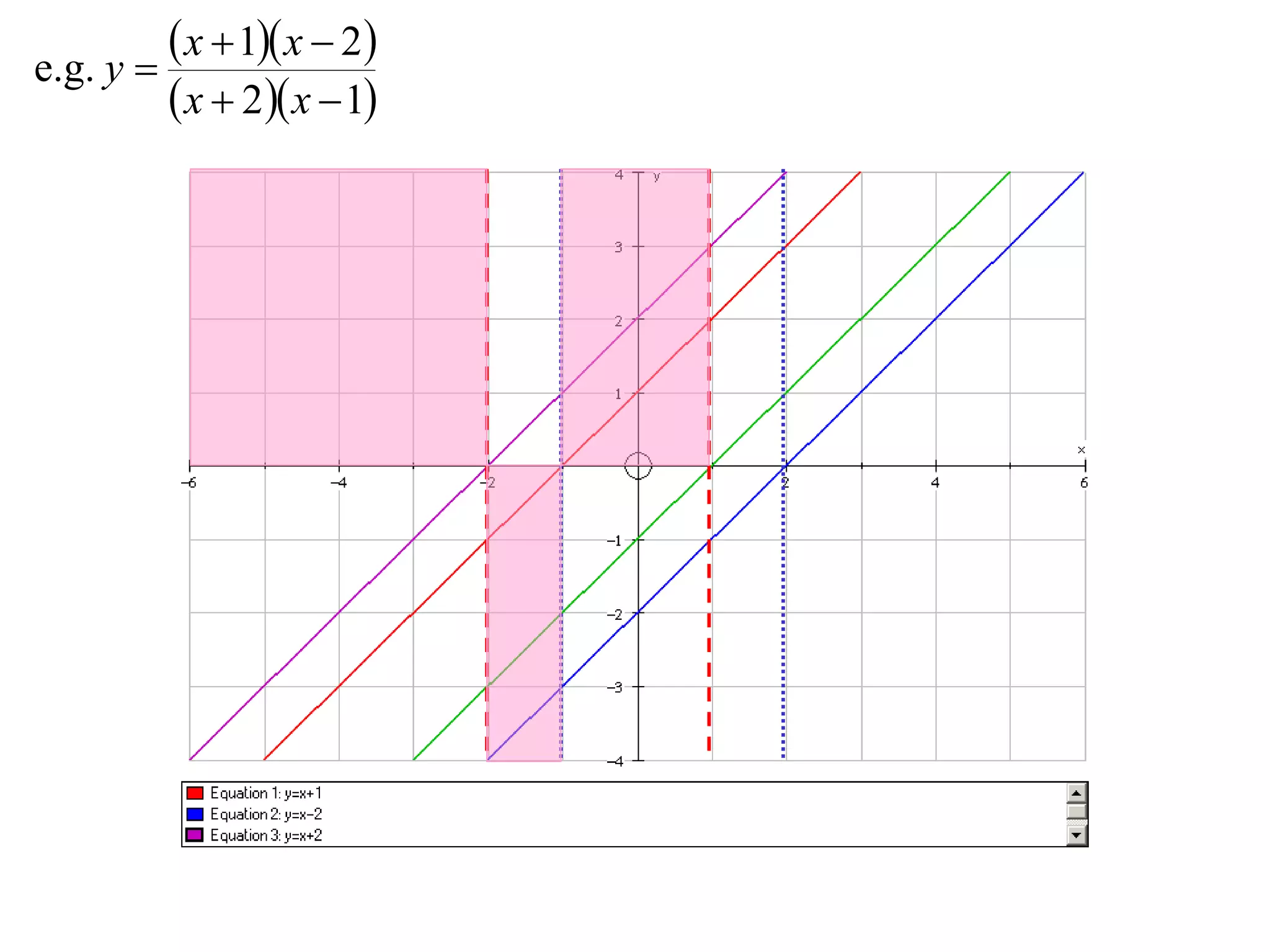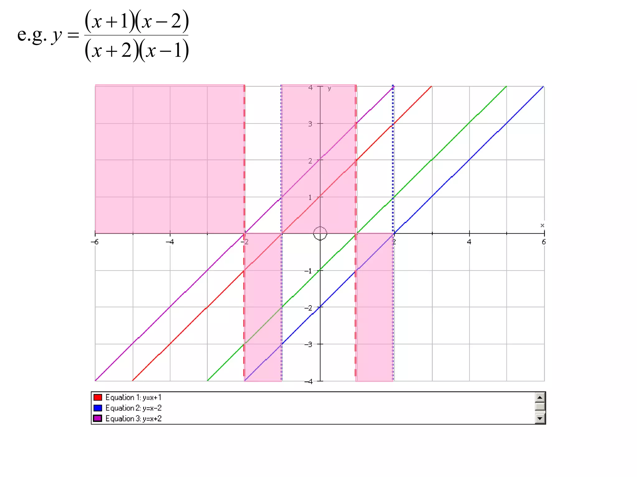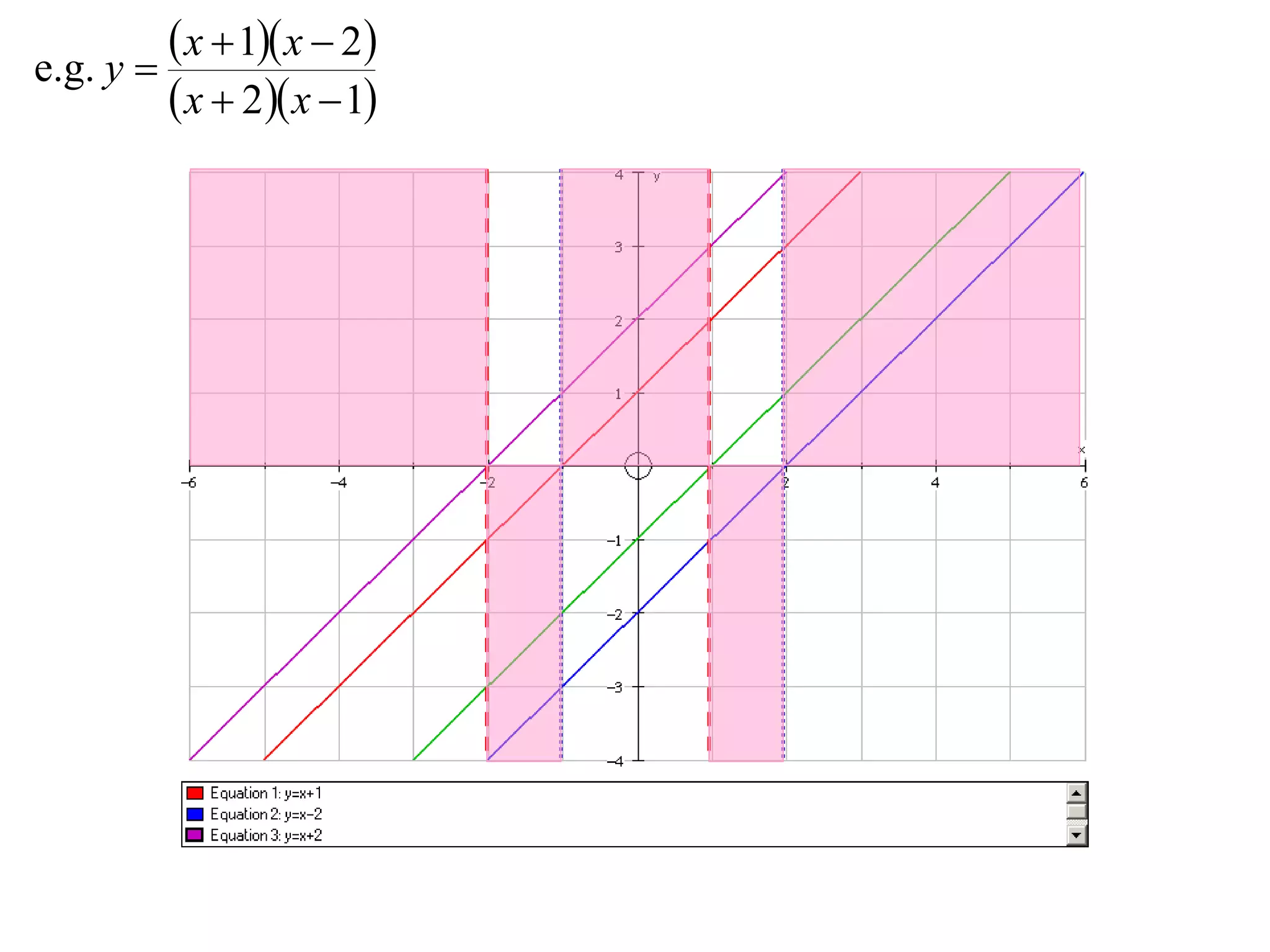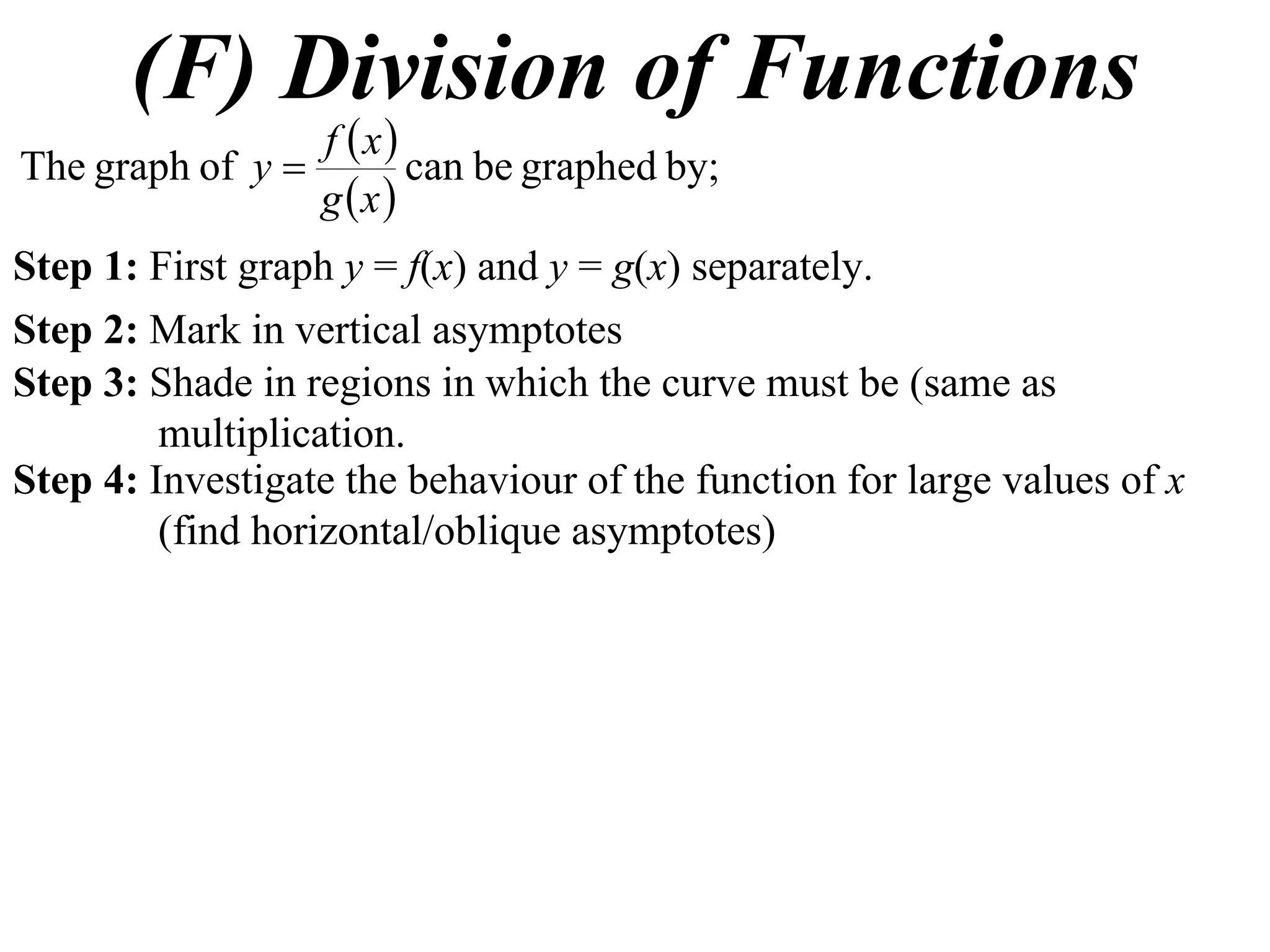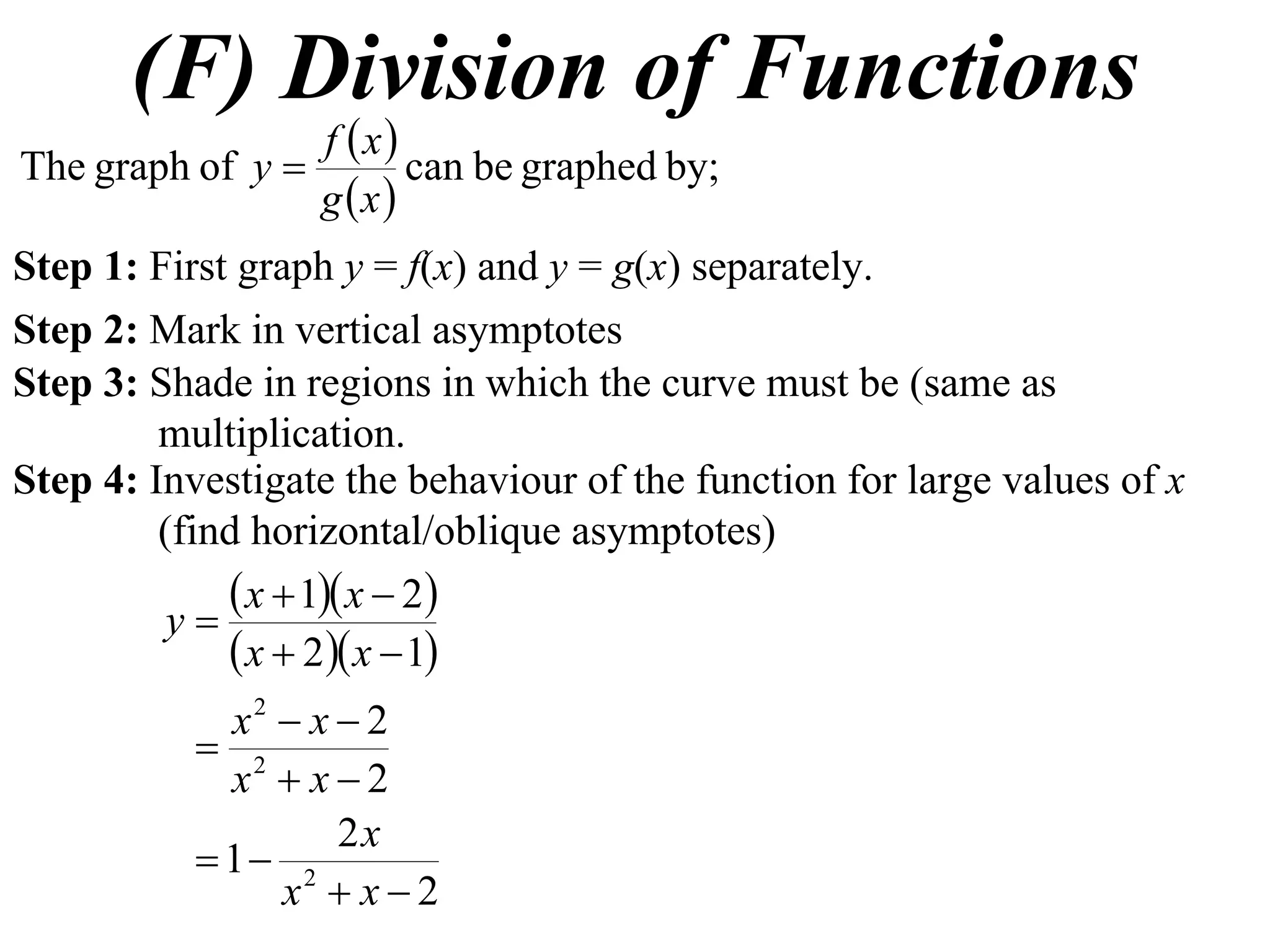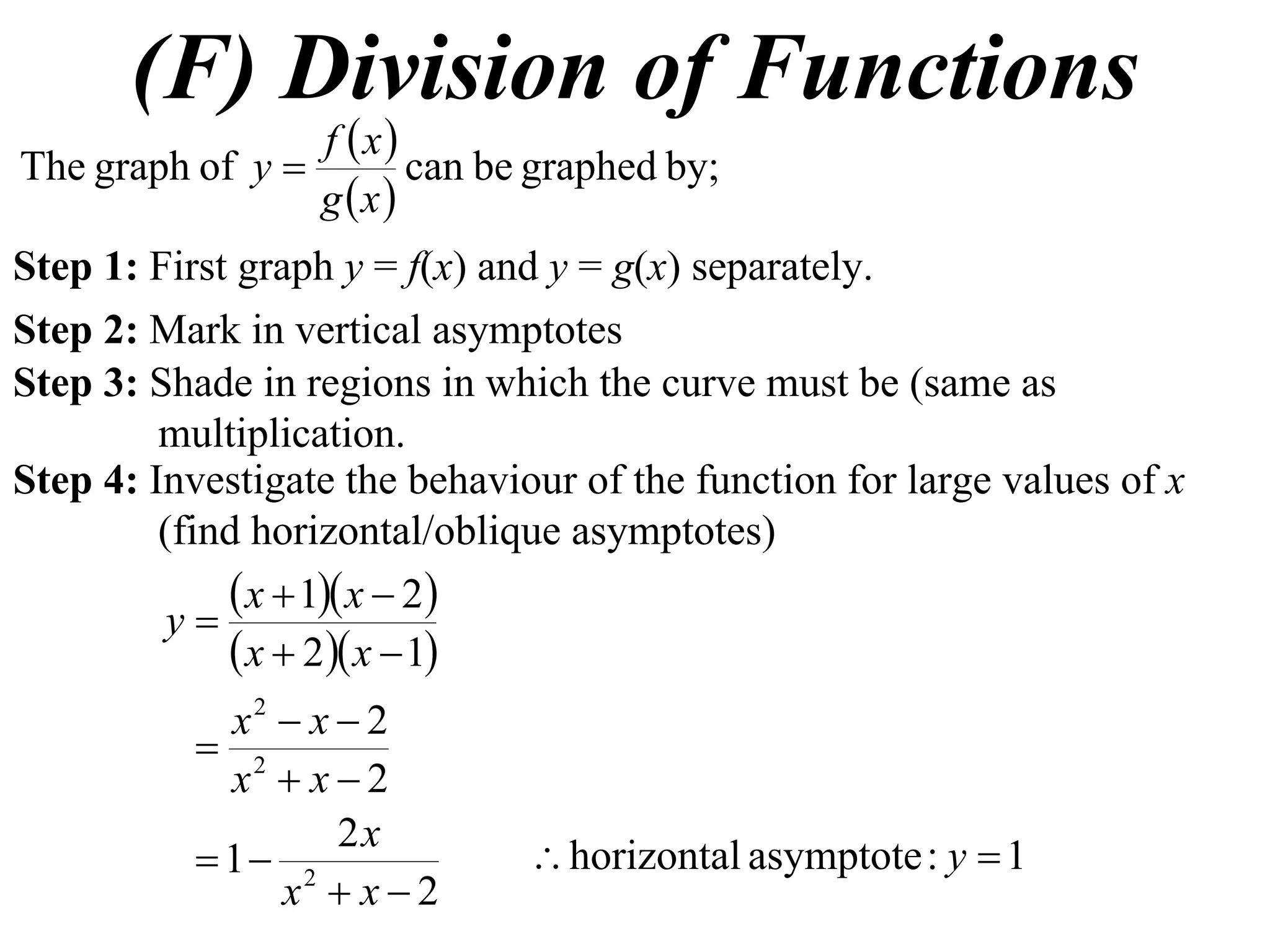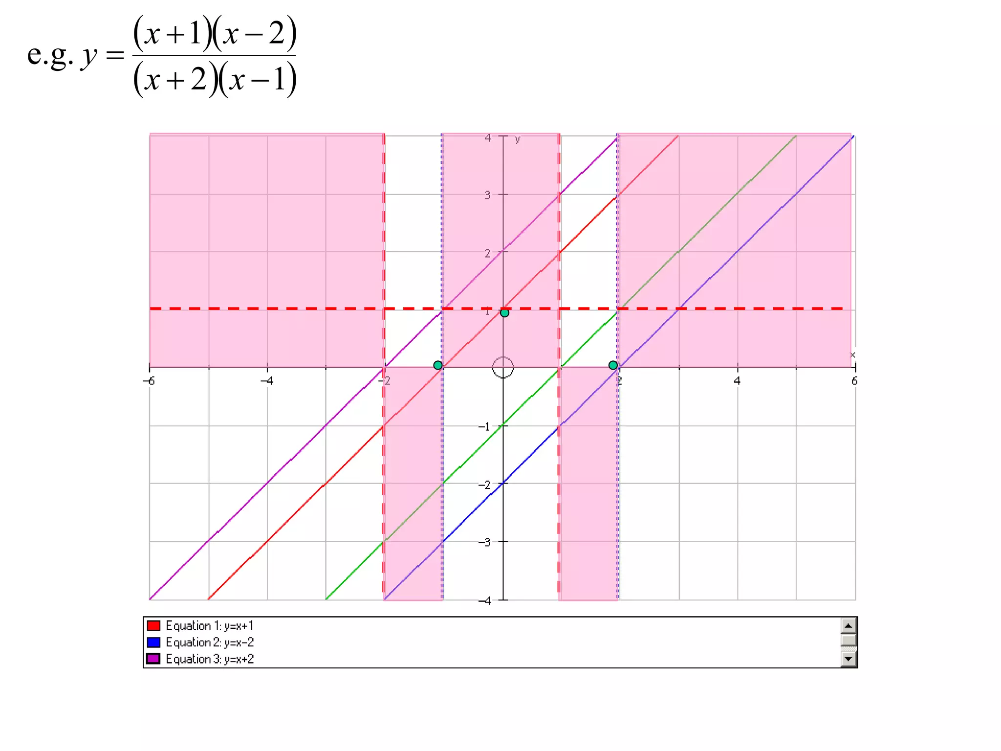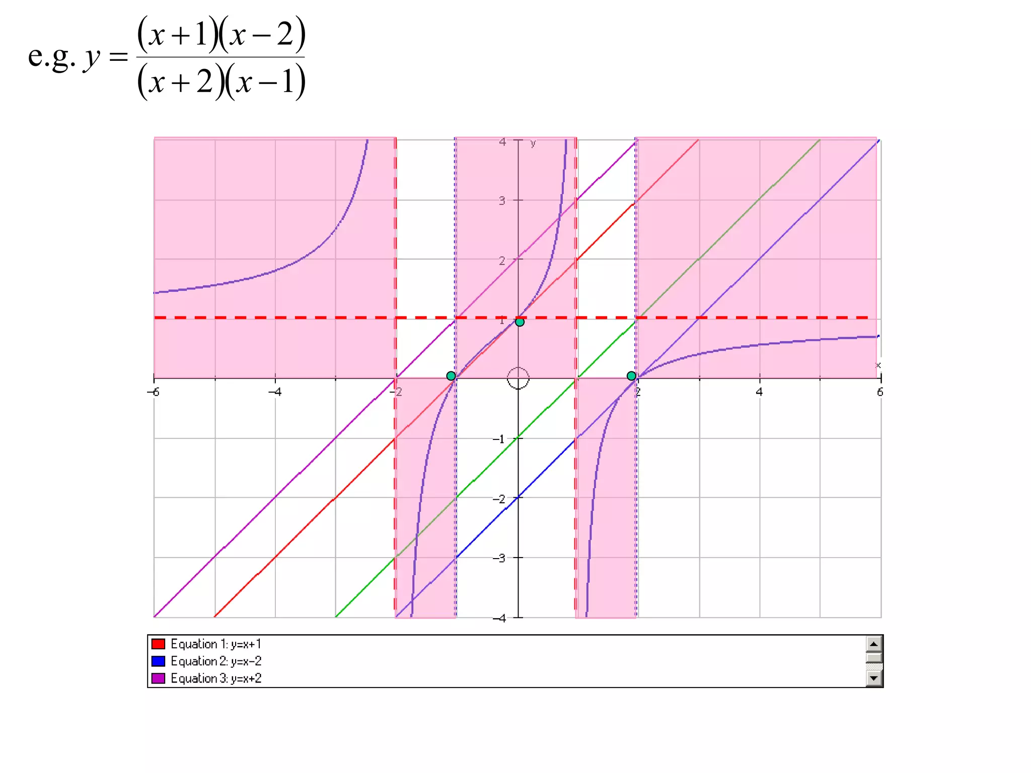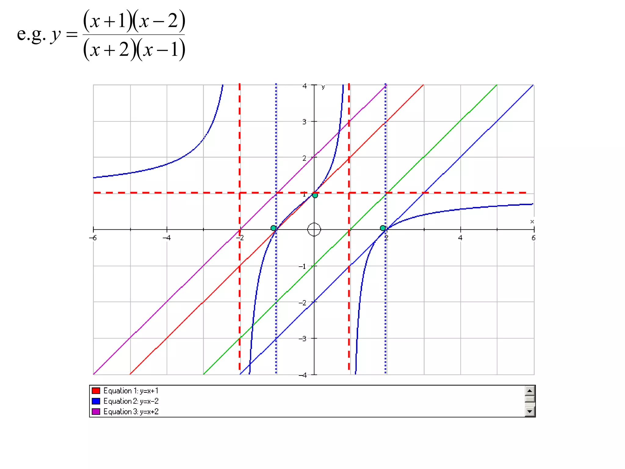- Division graphs are made by first graphing the numerator and denominator, then finding vertical and horizontal asymptotes and shading regions to determine the curve.

1. (D) Addition & Subtraction of
Ordinates

2. (D) Addition & Subtraction of
Ordinatesy = f(x) + g(x) can be graphed by first graphing y = f(x) and y = g(x)
separately and then adding their ordinates together.

3. (D) Addition & Subtraction of
Ordinatesy = f(x) + g(x) can be graphed by first graphing y = f(x) and y = g(x)
separately and then adding their ordinates together.
NOTE: First locate points on y = f(x) + g(x) corresponding to f(x)=0 and
g(x)=0, then plot further points by addition and subtraction of ordinates
and finally locate the position of stationary points.

4. (D) Addition & Subtraction of
Ordinatesy = f(x) + g(x) can be graphed by first graphing y = f(x) and y = g(x)
separately and then adding their ordinates together.
NOTE: First locate points on y = f(x) + g(x) corresponding to f(x)=0 and
g(x)=0, then plot further points by addition and subtraction of ordinates
and finally locate the position of stationary points.
x
xy
1
e.g. 

5. (D) Addition & Subtraction of
Ordinatesy = f(x) + g(x) can be graphed by first graphing y = f(x) and y = g(x)
separately and then adding their ordinates together.
y
x
NOTE: First locate points on y = f(x) + g(x) corresponding to f(x)=0 and
g(x)=0, then plot further points by addition and subtraction of ordinates
and finally locate the position of stationary points.
x
xy
1
e.g. 
xy 
x
y
1


6. (D) Addition & Subtraction of
Ordinatesy = f(x) + g(x) can be graphed by first graphing y = f(x) and y = g(x)
separately and then adding their ordinates together.
y
x
NOTE: First locate points on y = f(x) + g(x) corresponding to f(x)=0 and
g(x)=0, then plot further points by addition and subtraction of ordinates
and finally locate the position of stationary points.
x
xy
1
e.g. 
xy 
x
y
1


7. (D) Addition & Subtraction of
Ordinatesy = f(x) + g(x) can be graphed by first graphing y = f(x) and y = g(x)
separately and then adding their ordinates together.
y
x
NOTE: First locate points on y = f(x) + g(x) corresponding to f(x)=0 and
g(x)=0, then plot further points by addition and subtraction of ordinates
and finally locate the position of stationary points.
x
xy
1
e.g. 
xy 
x
y
1

x
xy
1


8. y = f(x) – g(x) can be graphed by first graphing y = f(x) and y = – g(x)
separately and then adding the ordinates together.

9. y = f(x) – g(x) can be graphed by first graphing y = f(x) and y = – g(x)
separately and then adding the ordinates together.
xxy sine.g. 

10. y = f(x) – g(x) can be graphed by first graphing y = f(x) and y = – g(x)
separately and then adding the ordinates together.
xxy sine.g. 

11. y = f(x) – g(x) can be graphed by first graphing y = f(x) and y = – g(x)
separately and then adding the ordinates together.
xxy sine.g. 

12. y = f(x) – g(x) can be graphed by first graphing y = f(x) and y = – g(x)
separately and then adding the ordinates together.
xxy sine.g. 

13. y = f(x) – g(x) can be graphed by first graphing y = f(x) and y = – g(x)
separately and then adding the ordinates together.
xxy sine.g. 

14. y = f(x) – g(x) can be graphed by first graphing y = f(x) and y = – g(x)
separately and then adding the ordinates together.
xxy sine.g. 

15. (E) Multiplication of Functions
The graph of y = f(x). g(x) can be graphed by first graphing y = f(x) and
y= g(x) separately and then examining the sign of the product. Special
note needs to be made of points where f(x) = 0 or 1, or g(x) = 0 or 1.
NOTE: The regions on the number plane through which the graph must
pass should be shaded in as the first step.

16.   32
11e.g.  xxxy

17.   32
11e.g.  xxxy

18.   32
11e.g.  xxxy

19.   32
11e.g.  xxxy

20.   32
11e.g.  xxxy

21.   32
11e.g.  xxxy

22.   32
11e.g.  xxxy

23.   32
11e.g.  xxxy

24.   32
11e.g.  xxxy

25. (F) Division of Functions
 
 
by;graphedbecanofgraphThe
xg
xf
y 

26. (F) Division of Functions
 
 
by;graphedbecanofgraphThe
xg
xf
y 
Step 1: First graph y = f(x) and y = g(x) separately.

27.   
  12
21
e.g.



xx
xx
y

28.   
  12
21
e.g.



xx
xx
y

29. (F) Division of Functions
 
 
by;graphedbecanofgraphThe
xg
xf
y 
Step 1: First graph y = f(x) and y = g(x) separately.
Step 2: Mark in vertical asymptotes

30.   
  12
21
e.g.



xx
xx
y

31. (F) Division of Functions
 
 
by;graphedbecanofgraphThe
xg
xf
y 
Step 1: First graph y = f(x) and y = g(x) separately.
Step 2: Mark in vertical asymptotes
Step 3: Shade in regions in which the curve must be (same as
multiplication.

32.   
  12
21
e.g.



xx
xx
y

33.   
  12
21
e.g.



xx
xx
y

34.   
  12
21
e.g.



xx
xx
y

35.   
  12
21
e.g.



xx
xx
y

36.   
  12
21
e.g.



xx
xx
y

37.   
  12
21
e.g.



xx
xx
y

38.   
  12
21
e.g.



xx
xx
y

39. (F) Division of Functions
 
 
by;graphedbecanofgraphThe
xg
xf
y 
Step 1: First graph y = f(x) and y = g(x) separately.
Step 2: Mark in vertical asymptotes
Step 3: Shade in regions in which the curve must be (same as
multiplication.
Step 4: Investigate the behaviour of the function for large values of x
(find horizontal/oblique asymptotes)

40. (F) Division of Functions
 
 
by;graphedbecanofgraphThe
xg
xf
y 
Step 1: First graph y = f(x) and y = g(x) separately.
Step 2: Mark in vertical asymptotes
Step 3: Shade in regions in which the curve must be (same as
multiplication.
Step 4: Investigate the behaviour of the function for large values of x
(find horizontal/oblique asymptotes)
  
  
2
2
1
2
2
12
21
2
2
2








xx
x
xx
xx
xx
xx
y

41. (F) Division of Functions
 
 
by;graphedbecanofgraphThe
xg
xf
y 
Step 1: First graph y = f(x) and y = g(x) separately.
Step 2: Mark in vertical asymptotes
Step 3: Shade in regions in which the curve must be (same as
multiplication.
Step 4: Investigate the behaviour of the function for large values of x
(find horizontal/oblique asymptotes)
  
  
2
2
1
2
2
12
21
2
2
2








xx
x
xx
xx
xx
xx
y
1:asymptotehorizontal  y

42.   
  12
21
e.g.



xx
xx
y

43.   
  12
21
e.g.



xx
xx
y

44.   
  12
21
e.g.



xx
xx
y