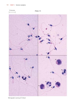
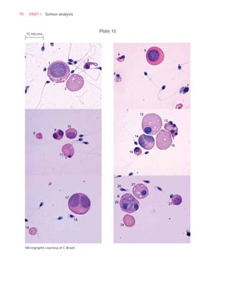
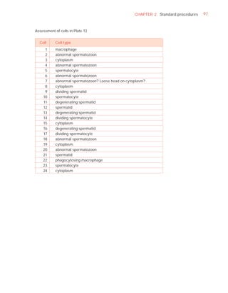
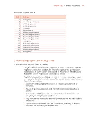
Downloaded 619 times
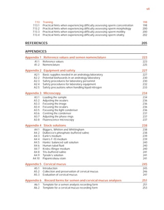
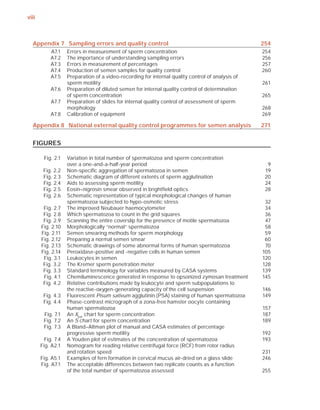
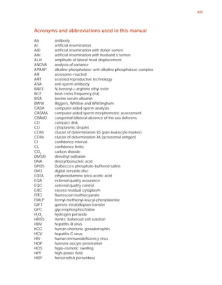
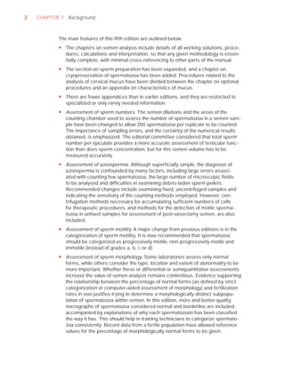


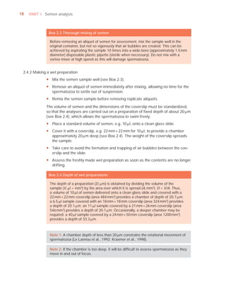
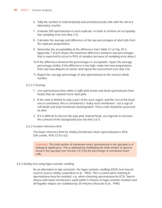
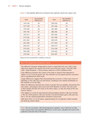
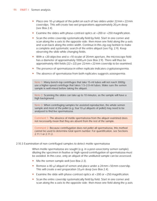
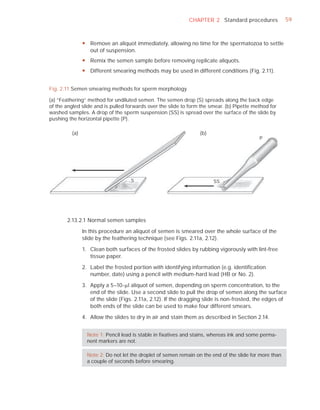

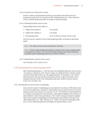
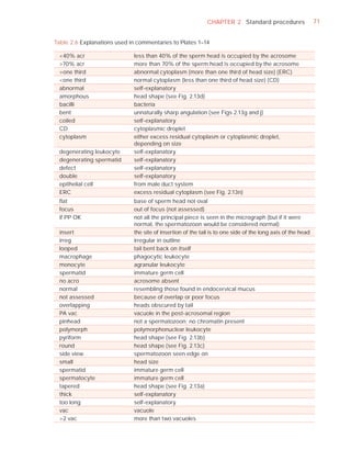

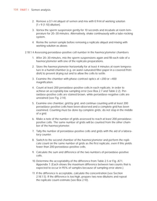

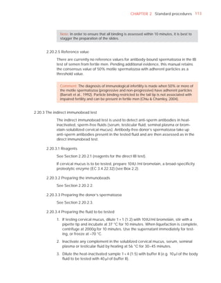
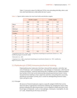
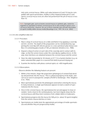

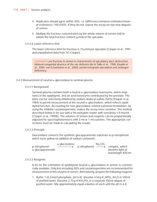
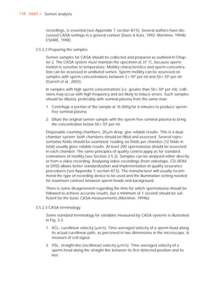
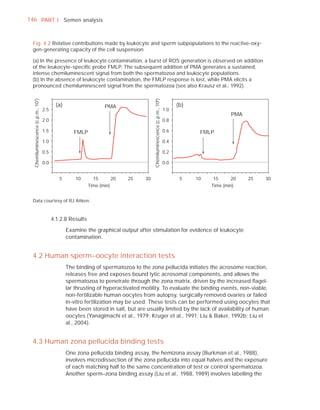
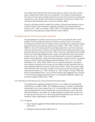
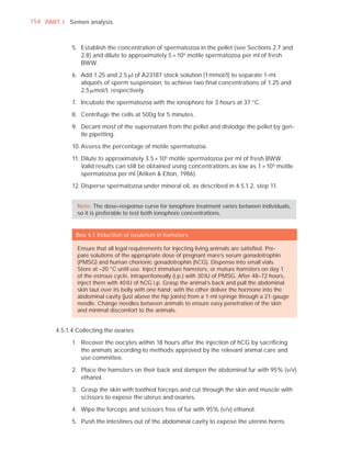


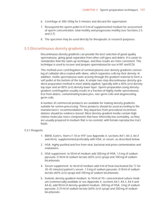
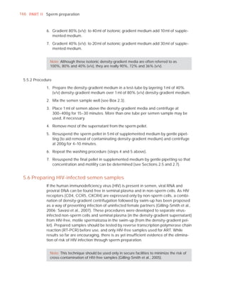
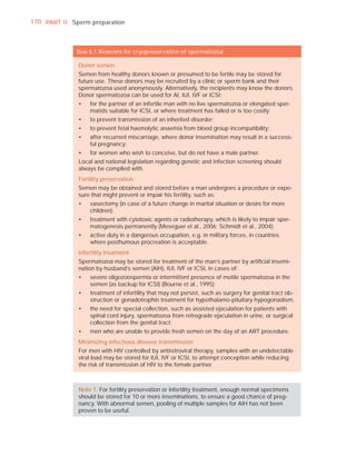
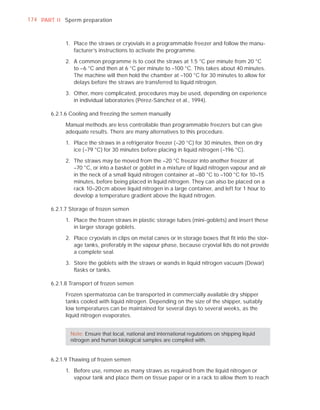


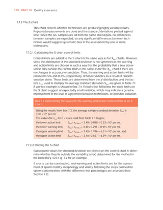
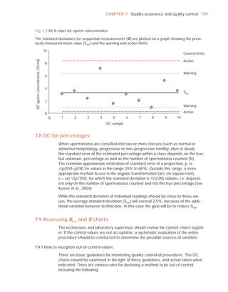

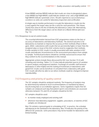
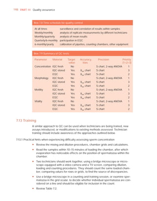


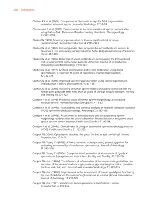

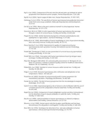


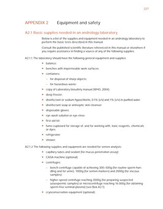
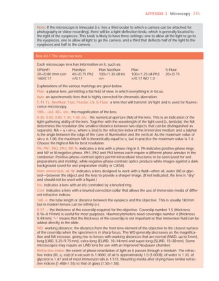

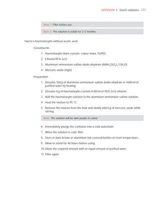
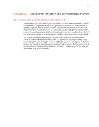
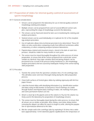
![252 APPENDIX 6 Record forms for semen and cervical mucus analyses
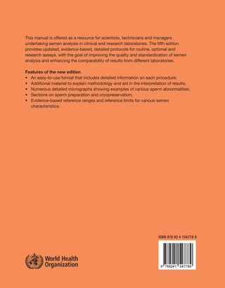
Name:
Code:
Date (day/month/year)
Collection (1, at laboratory; 2, at home)
Collection time (hour : minute)
Sample delivered (hour : minute)
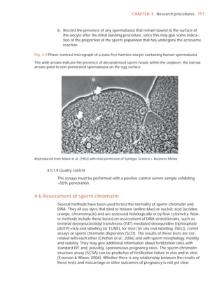
Analysis begun (hour : minute)
Patient
Abstinence time (days)
Medication
Difficulties in collection
Semen
Treatment (e.g. bromelain)
Complete sample? (1, complete; 2, incomplete)
Appearance (1, normal; 2, abnormal)
Viscosity (1, normal; 2, abnormal)
Liquefaction (1, normal; 2, abnormal) (minutes)
Agglutination (1–4, A–E)
pH [t7.2]
Volume (ml) [t1.5]
Spermatozoa
Total number (106 per ejaculate) [t39]
Concentration (106 per ml) [t15]
Error (%) if fewer than 400 cells counted
Vitality (% alive) [t58]
Total motile PR + NP (%) [t40]
Progressive PR (%) [t32]
Non-progressive NP (%)
Immotile IM (%)
Normal forms (%) [t4]
Abnormal heads (%)
Abnormal midpieces (%)
Abnormal principal pieces (%)
Excess residual cytoplasm (%)
Direct MAR-test IgG (%) (3 or 10 minute) [50]
Direct MAR-test IgA (%) (3 or 10 minute) [50]
Direct IB-test IgG (% with beads) [50]
Direct IB-test IgA (% with beads) [50]
Non-sperm cells
Peroxidase-positive cells, concentration (106 per ml) [1.0]
Accessory gland function
Zinc (µmol per ejaculate) [t2.4]
Fructose (µmol per ejaculate) [t13]
D-Glucosidase (neutral) (mU/ejaculate) [t20]
Technician:](https://image.slidesharecdn.com/whohumansemen5thed-110927054425-phpapp02/85/WHO-Human-Semen-Analysis-5th-ed-266-320.jpg)

This document is the fifth edition of the WHO laboratory manual for the examination and processing of human semen. It provides standardized procedures for semen analysis, including sample collection, initial macroscopic and microscopic examination, assessment of sperm motility, vitality, concentration, and morphology. The manual establishes reference values and diagnostic criteria and ensures uniformity in reporting results across laboratories worldwide.


