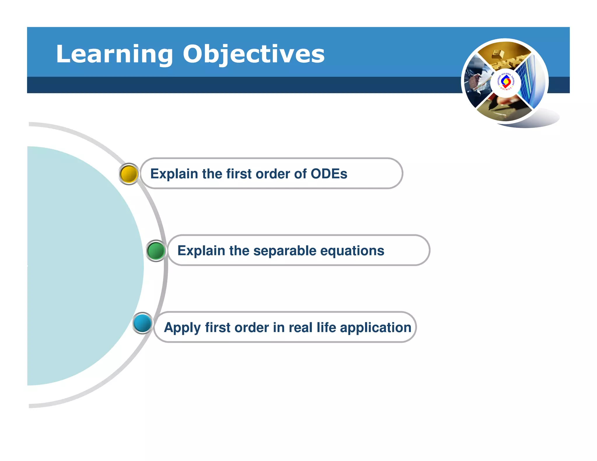
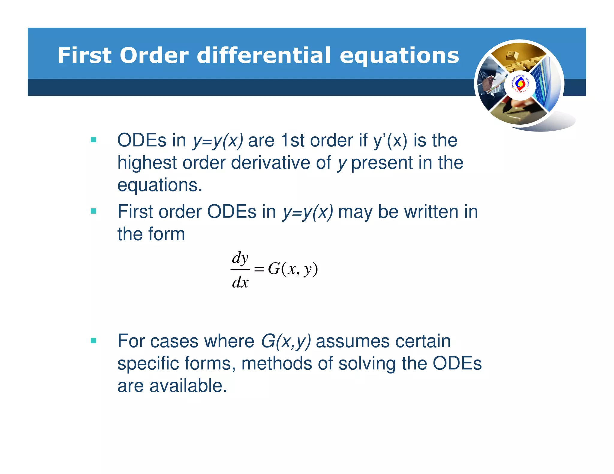
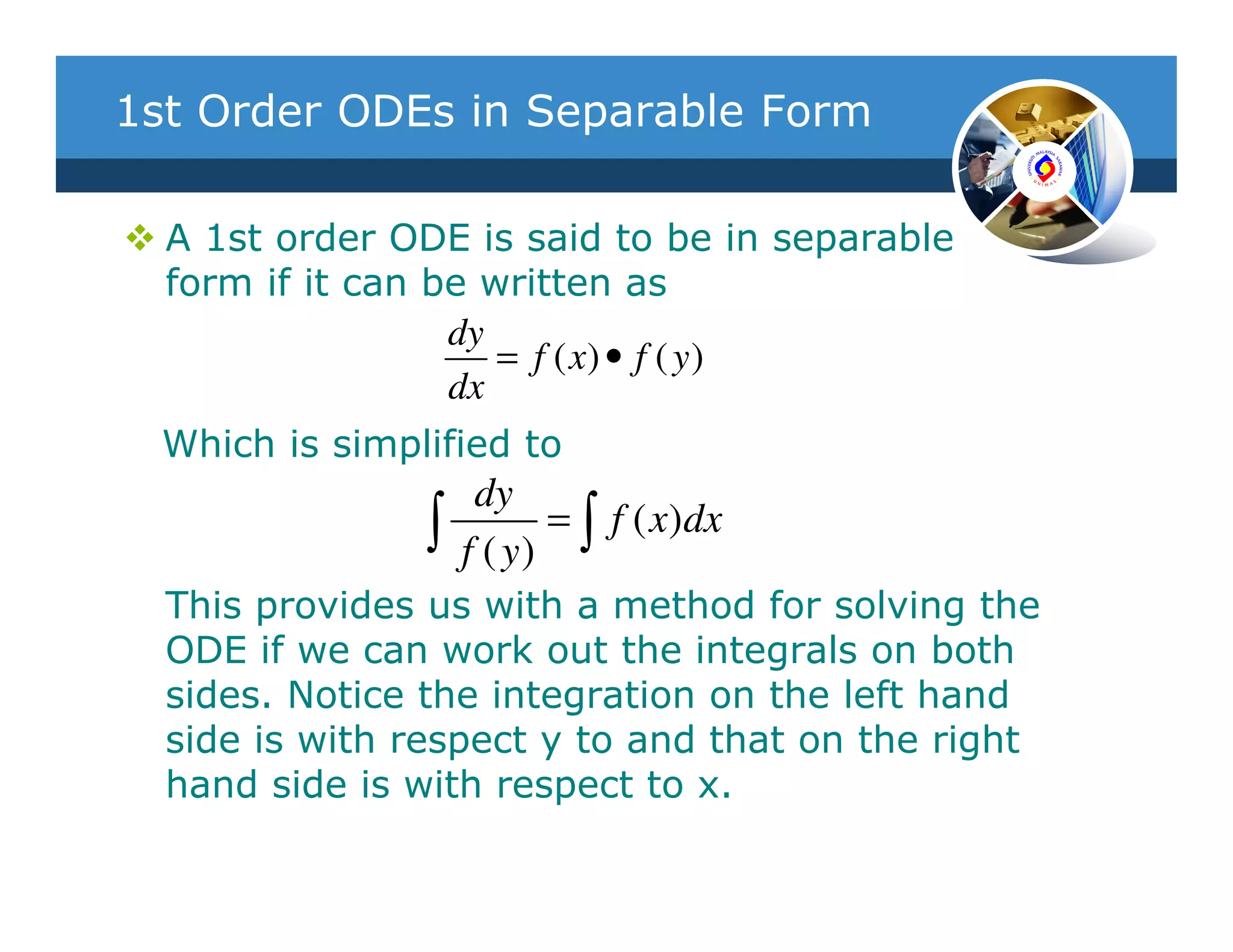
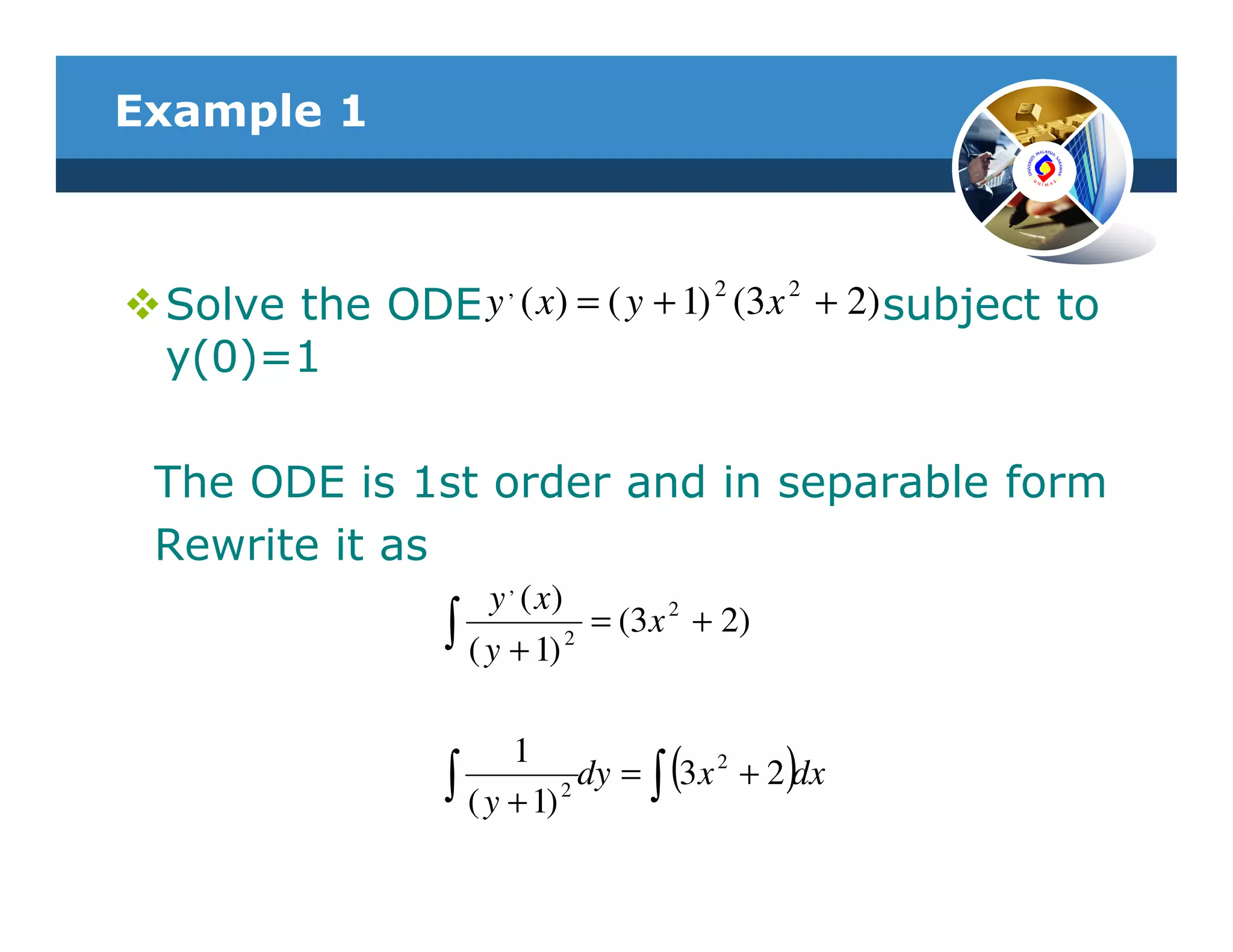
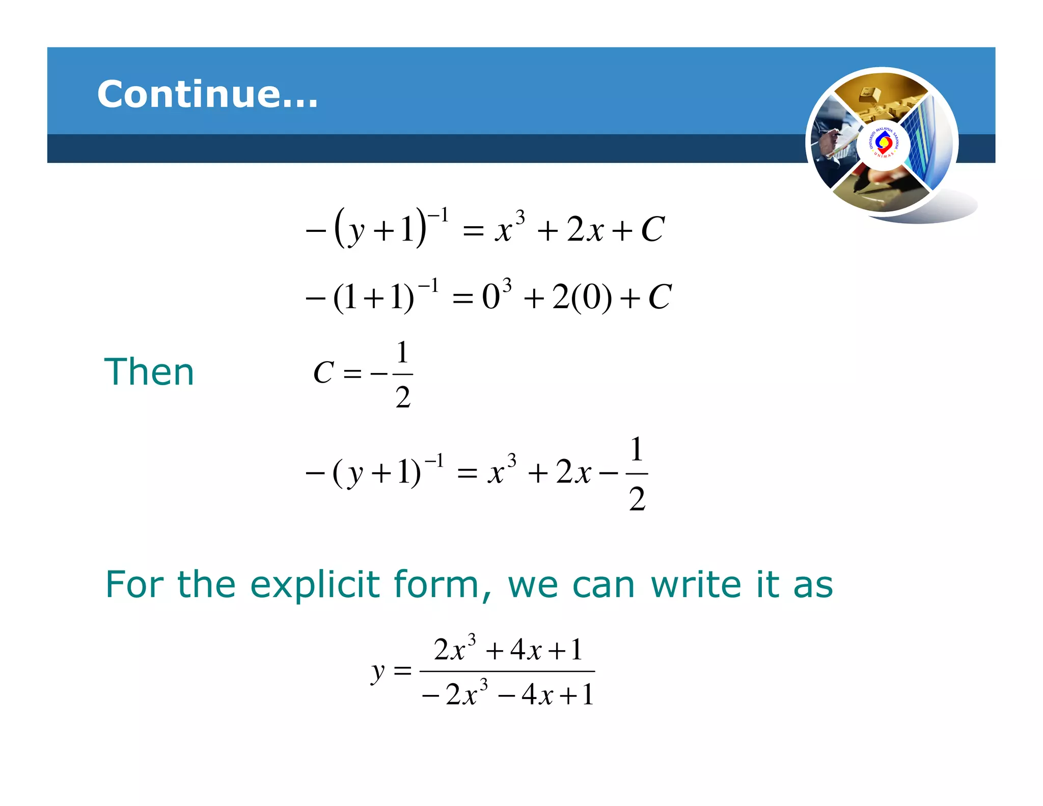
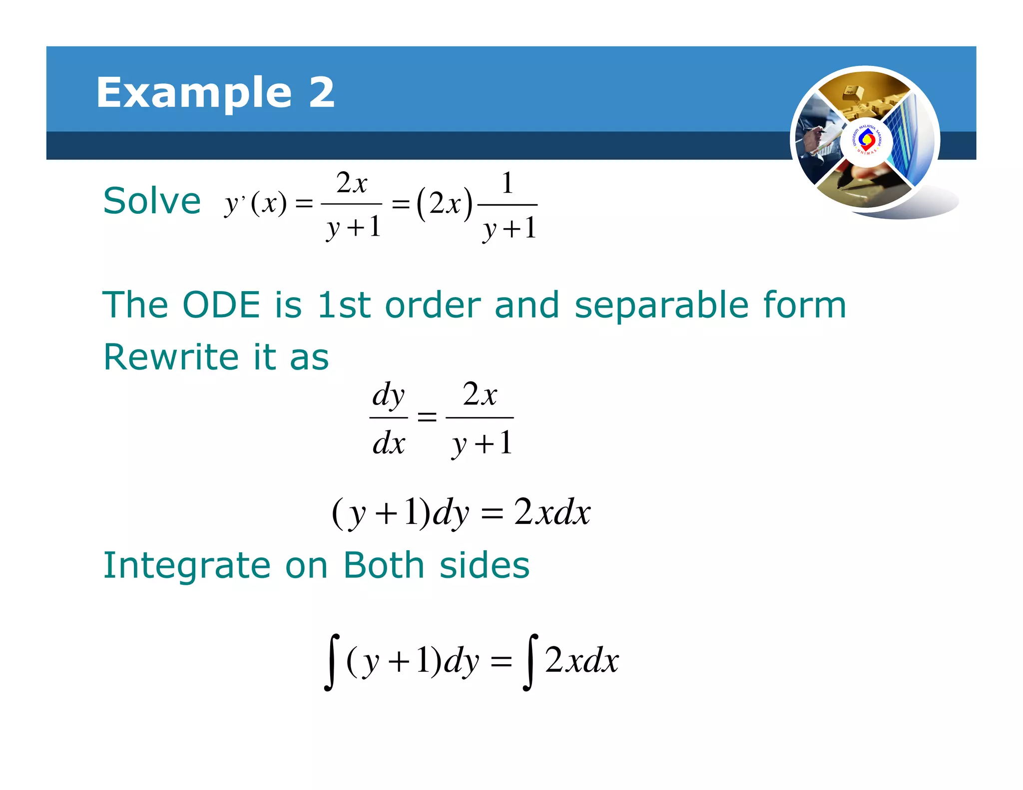
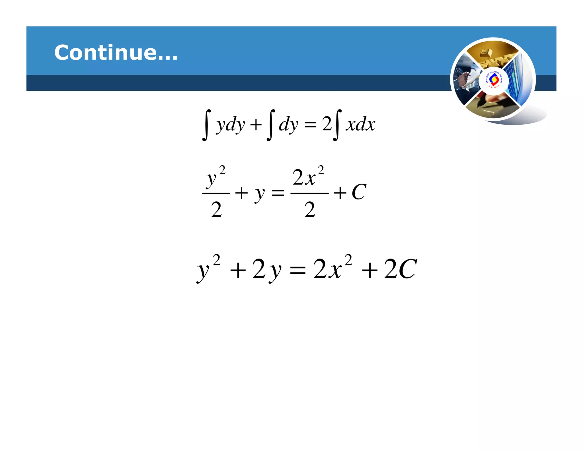
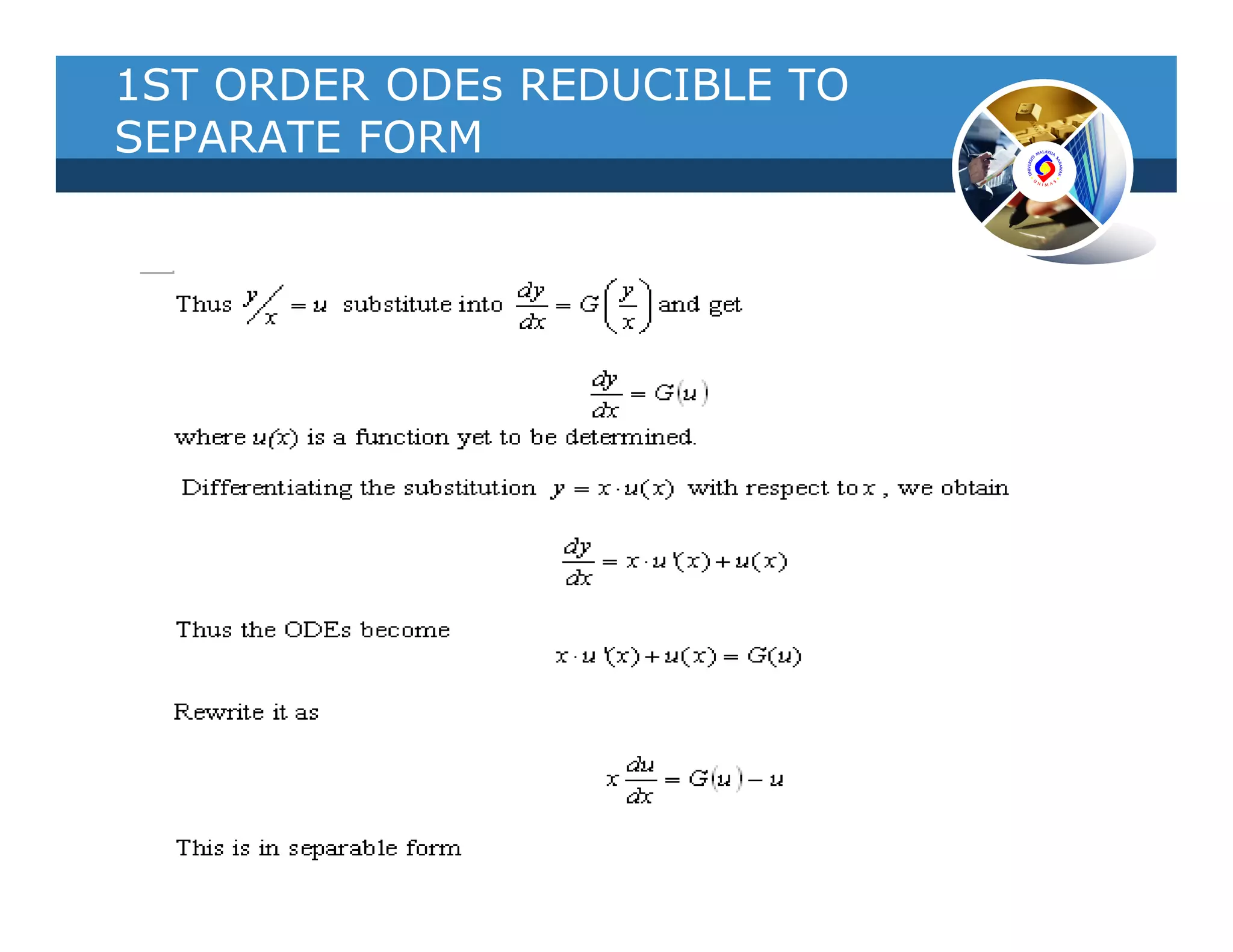
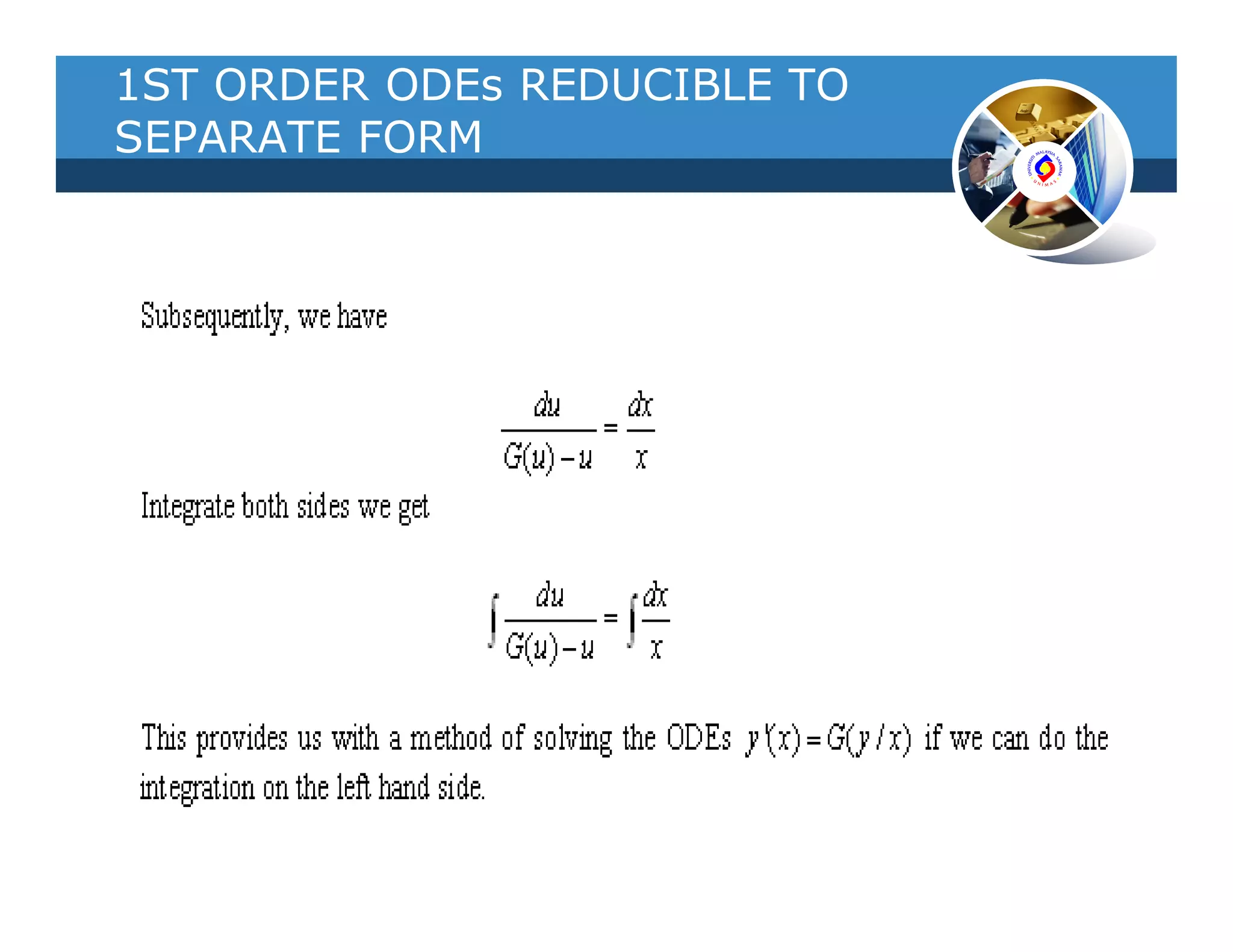
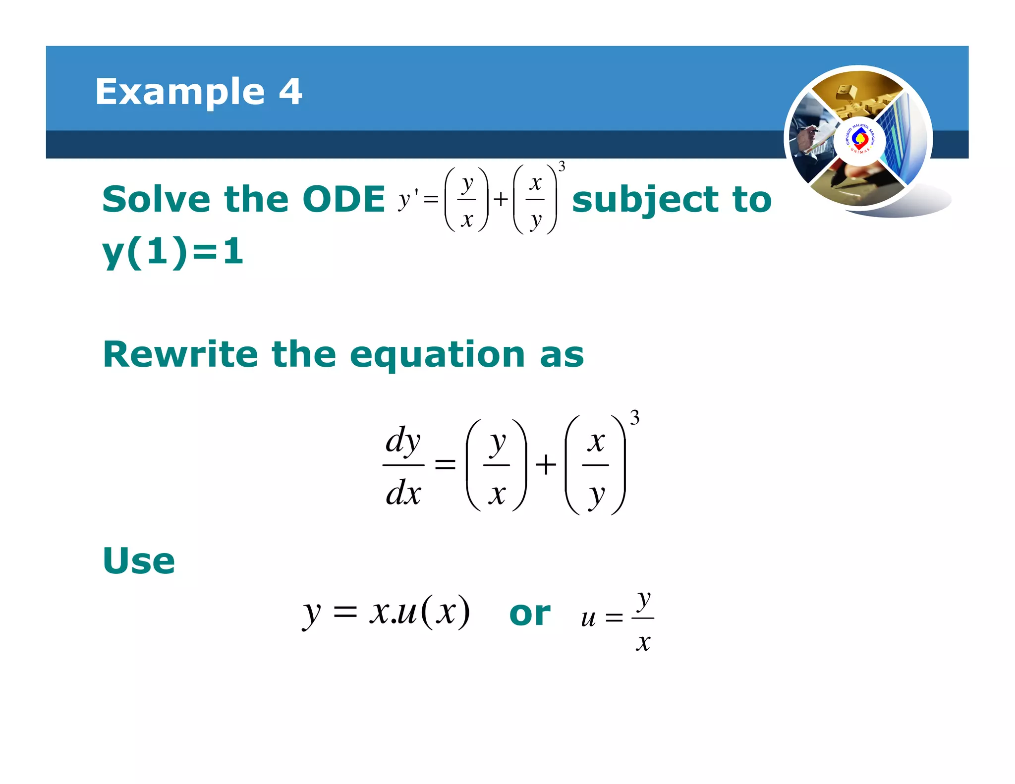
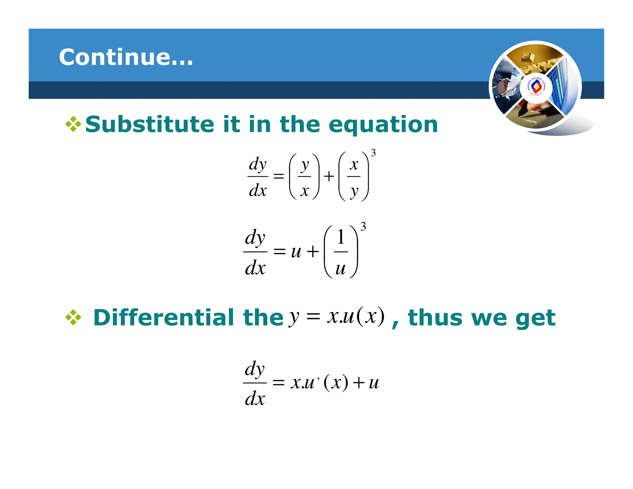
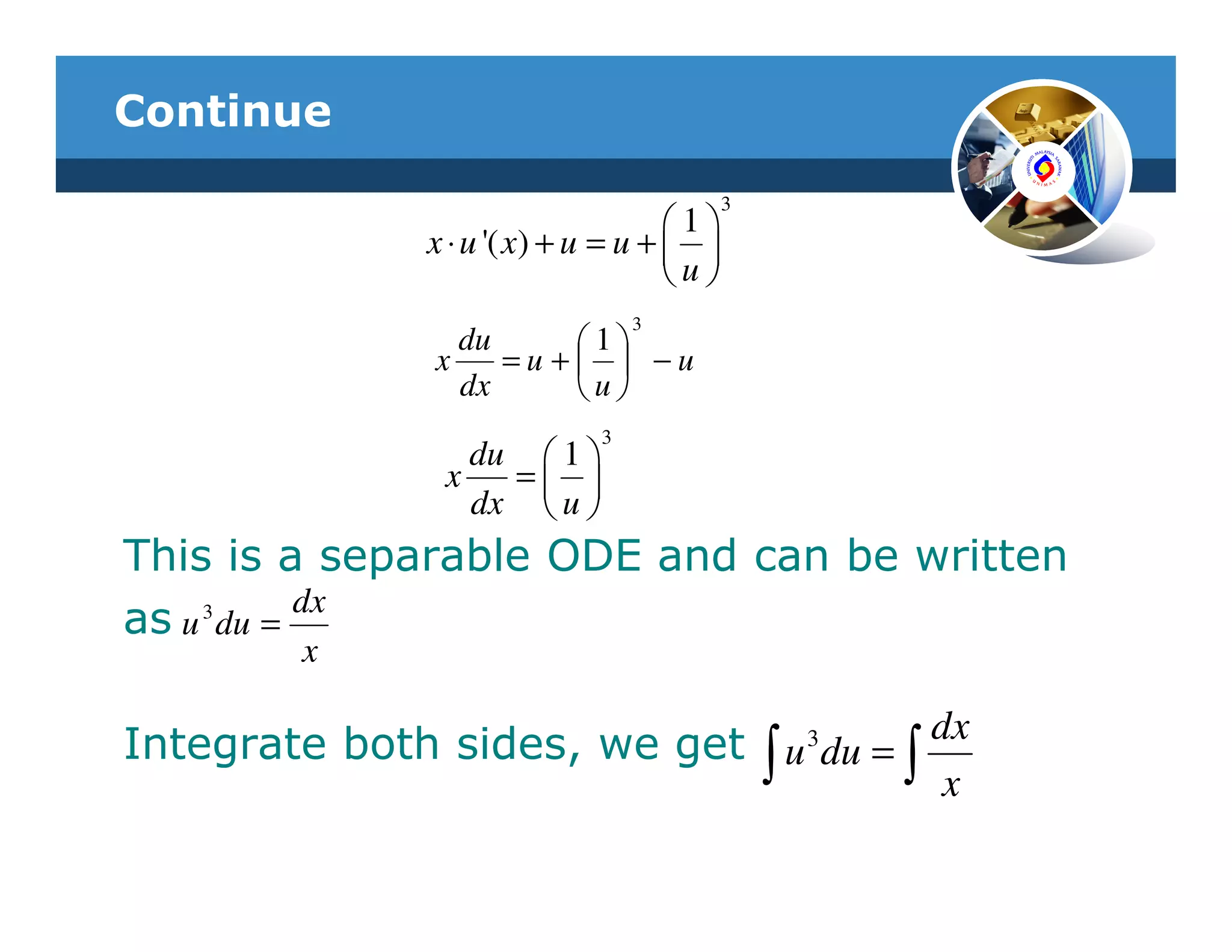
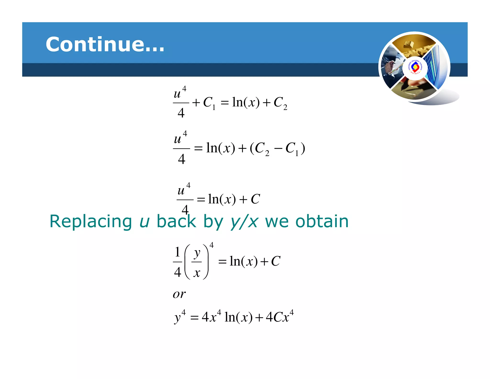
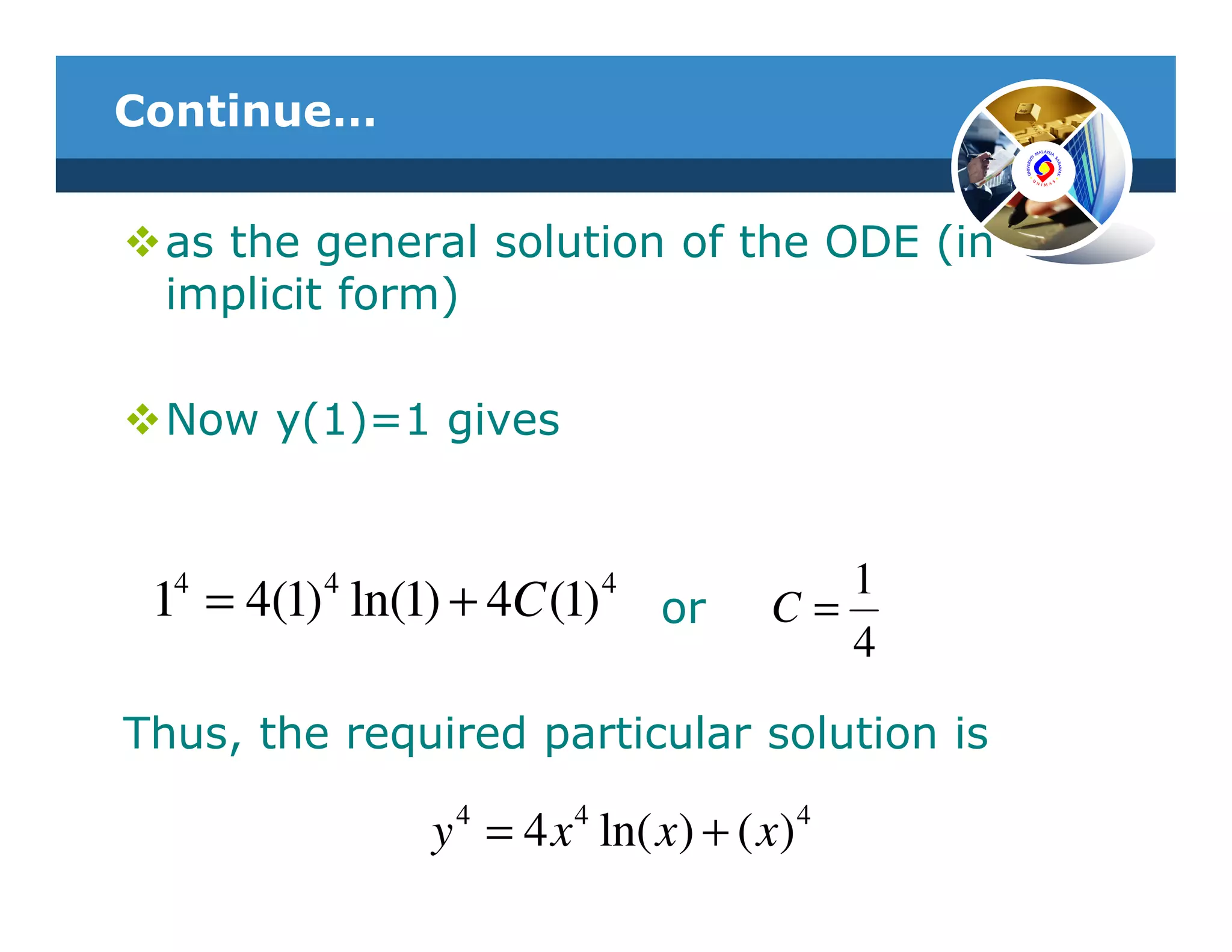
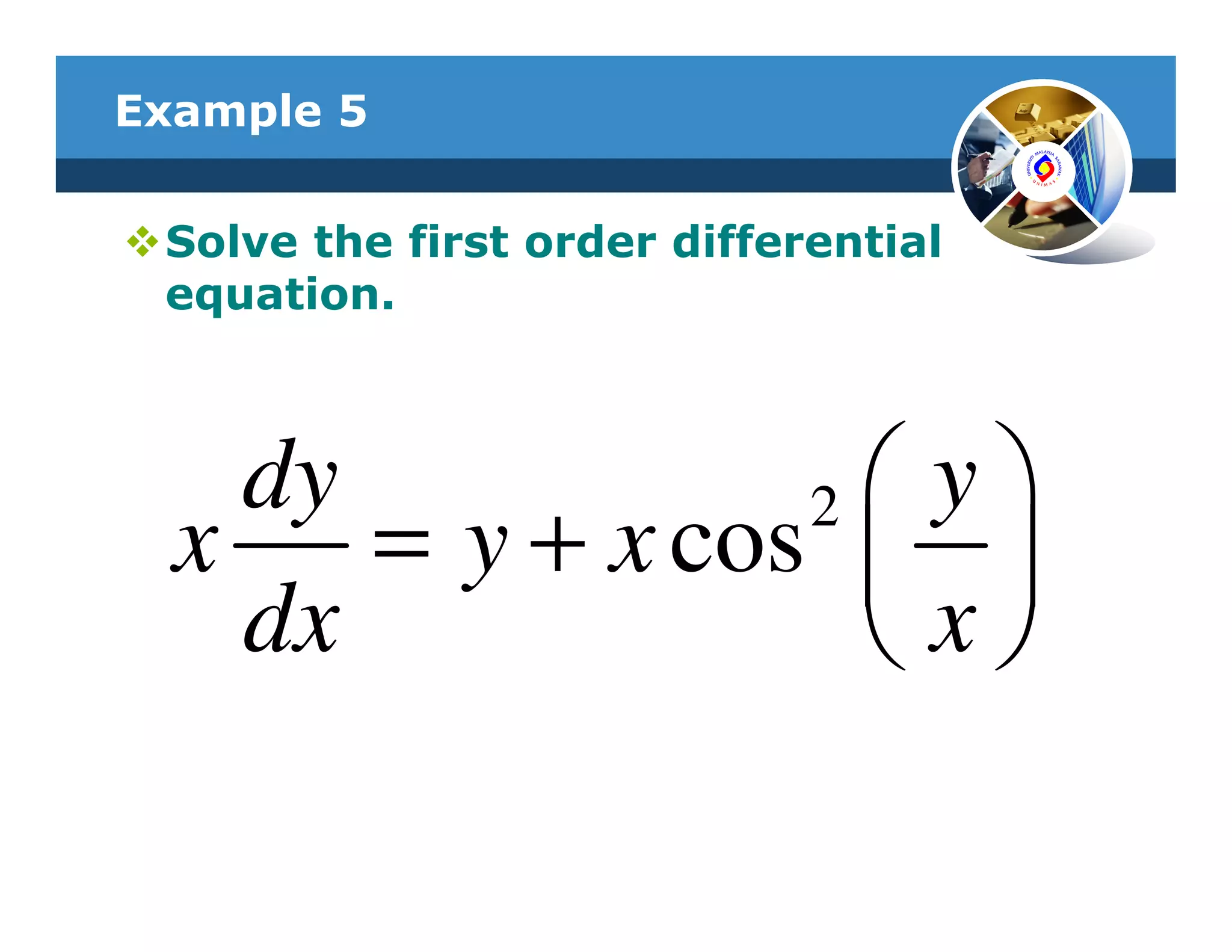
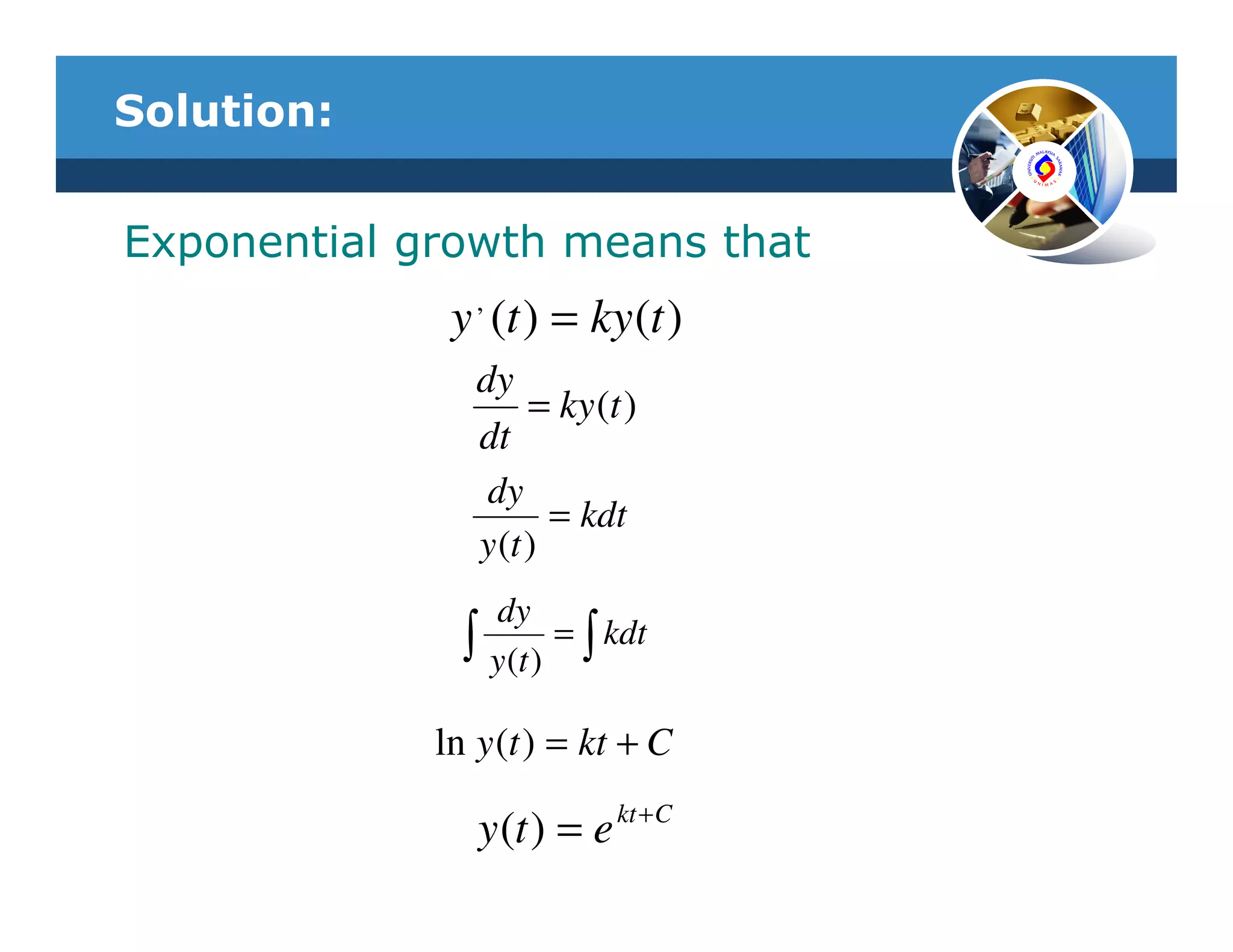
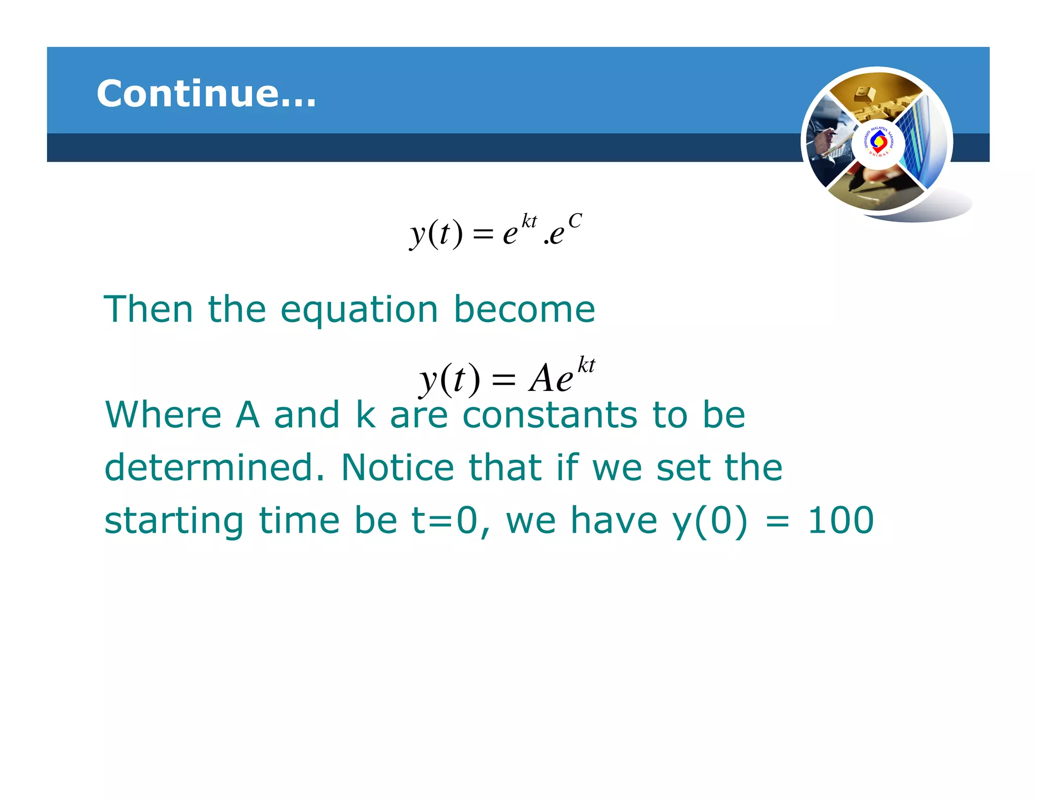
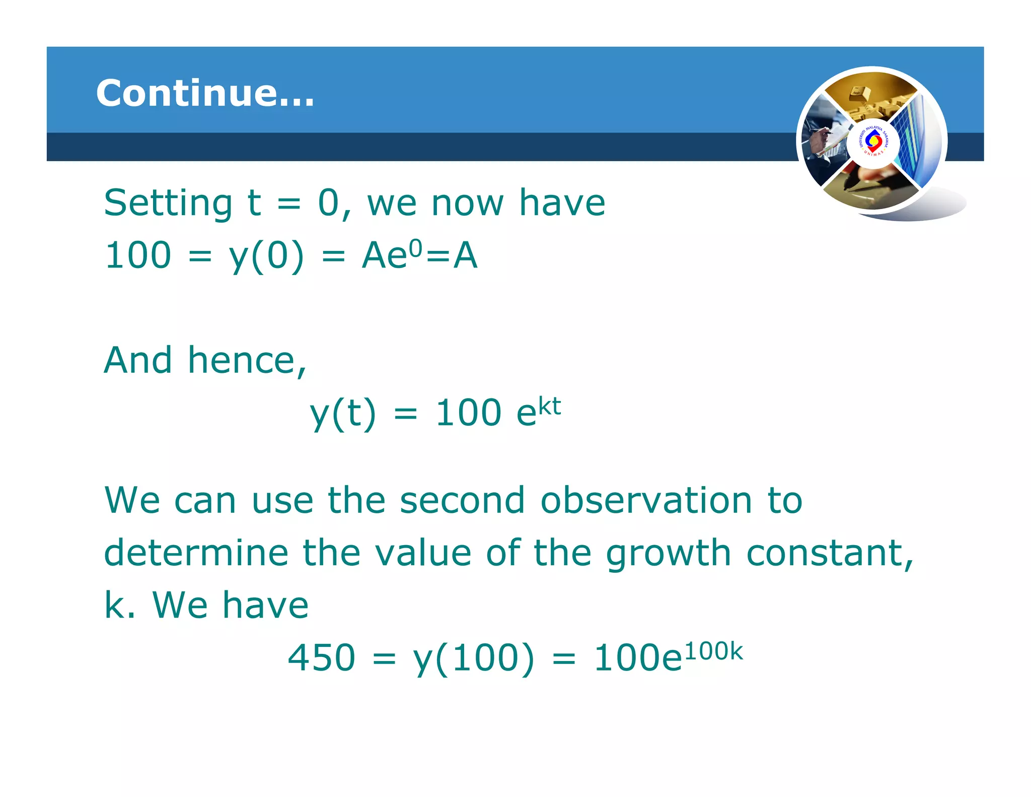
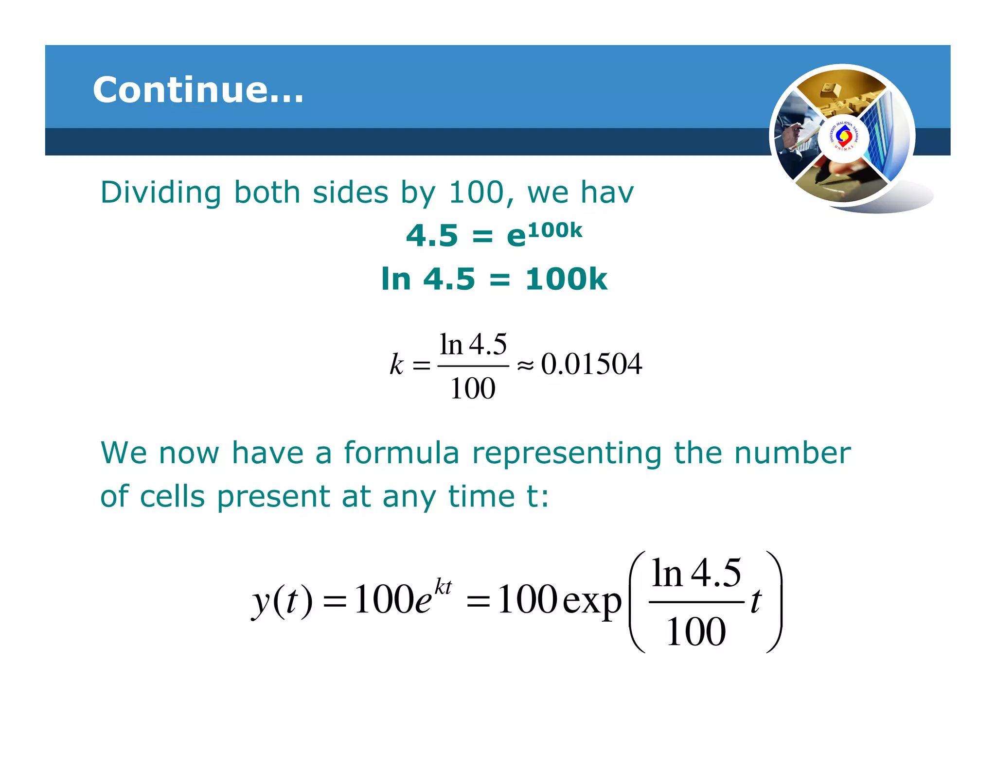
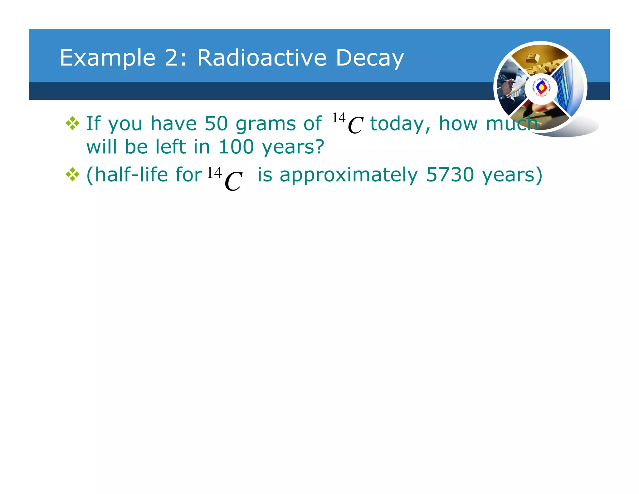
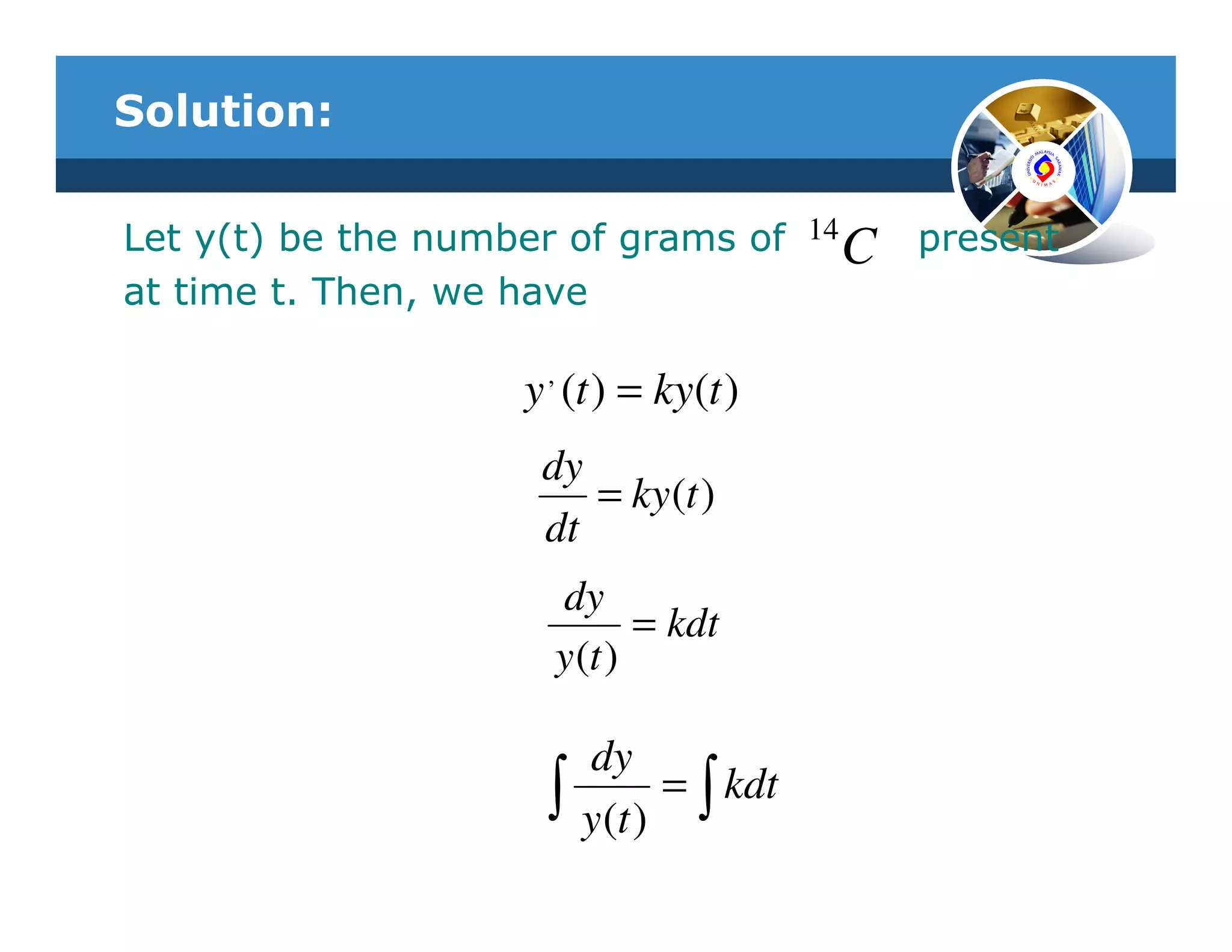
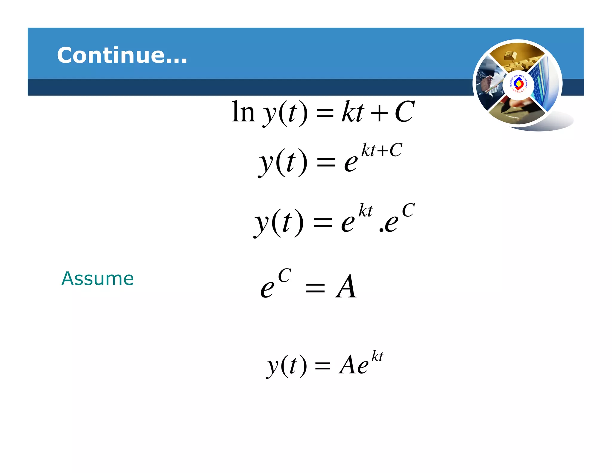
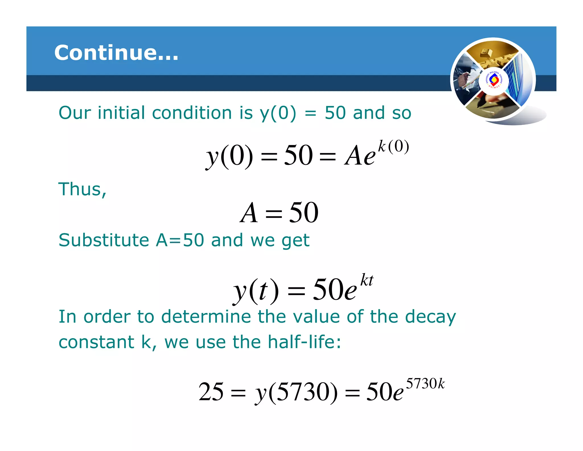
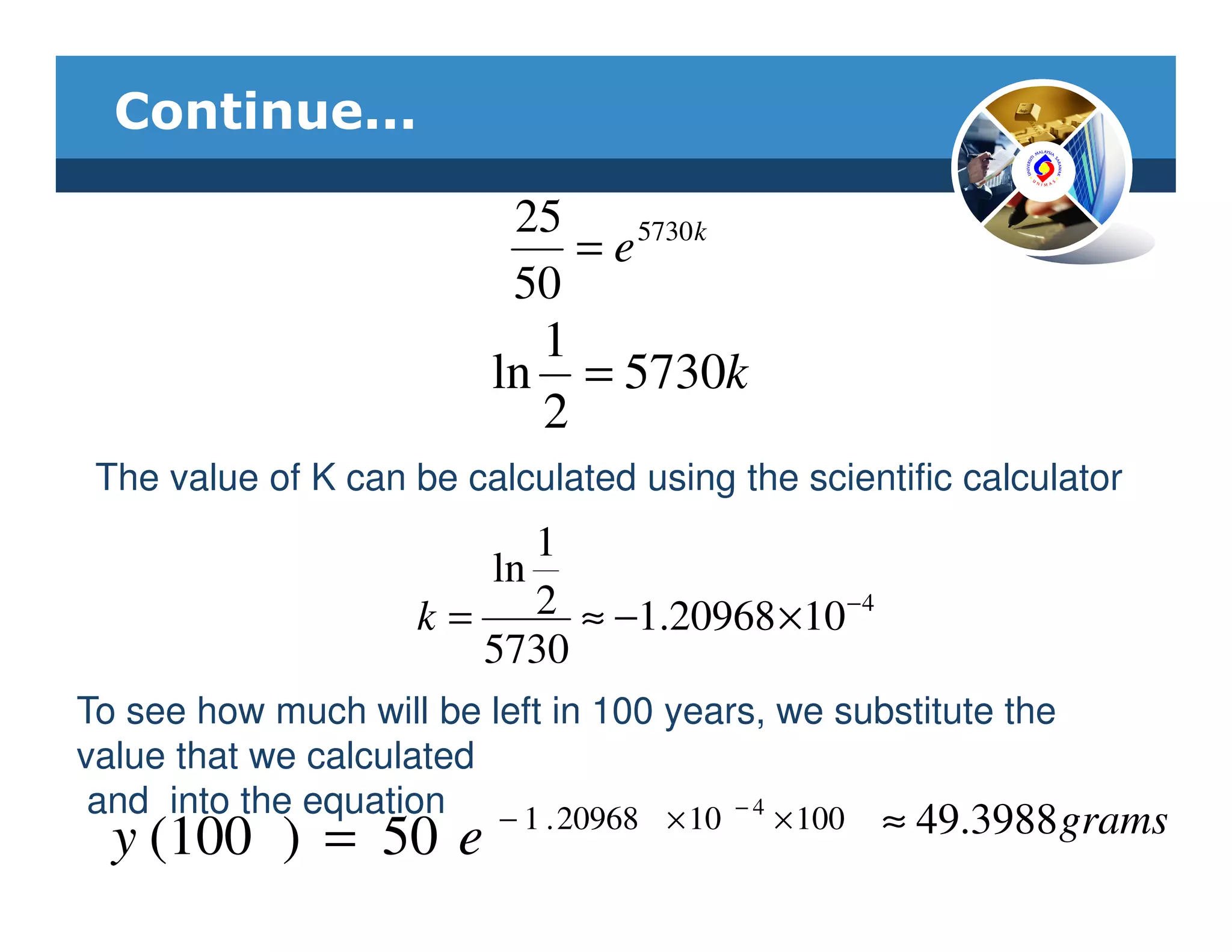
SlideShare a Scribd company logo
KNF1023
                                   Engineering
                                Mathematics II

                                   First Order ODEs
               Prepared By
              Annie ak Joseph


Prepared By
Annie ak Joseph                          Session 2008/2009
Learning Objectives


      Explain the first order of ODEs


          Explain the separable equations


        Apply first order in real life application
First Order differential equations


     ODEs in y=y(x) are 1st order if y’(x) is the
     highest order derivative of y present in the
     equations.
     First order ODEs in y=y(x) may be written in
     the form
                  dy
                     = G ( x, y )
                  dx


     For cases where G(x,y) assumes certain
     specific forms, methods of solving the ODEs
     are available.
1st Order ODEs in Separable Form

  A 1st order ODE is said to be in separable
  form if it can be written as
                  dy
                     = f ( x) • f ( y )
                  dx
  Which is simplified to
                     dy
                ∫   f ( y)
                           = ∫ f ( x)dx

  This provides us with a method for solving the
  ODE if we can work out the integrals on both
  sides. Notice the integration on the left hand
  side is with respect y to and that on the right
  hand side is with respect to x.
Example 1


 Solve the ODE y , ( x) = ( y + 1) 2 (3x 2 + 2) subject to
 y(0)=1

 The ODE is 1st order and in separable form
 Rewrite it as
                      y , ( x)
                  ∫ ( y + 1) 2 = (3 x 2 + 2)


                        1
                  ∫ ( y + 1) 2       (         )
                               dy = ∫ 3 x 2 + 2 dx
Continue…


                        −1
           − ( y + 1) = x 3 + 2 x + C
           − (1 + 1) −1 = 0 3 + 2(0) + C
               1
Then       C=−
               2
                        −1      3       1
           − ( y + 1)        = x + 2x −
                                        2

For the explicit form, we can write it as
                    2x3 + 4x + 1
                y=
                   − 2x3 − 4x + 1
Example 2

          ,     2x           1
Solve y ( x) =      = ( 2x)
               y +1         y +1

The ODE is 1st order and separable form
Rewrite it as
              dy   2x
                 =
              dx y + 1

                ( y + 1)dy = 2 xdx
Integrate on Both sides

                ∫ ( y + 1)dy = ∫ 2 xdx
Continue…


            ∫ ydy + ∫ dy = 2∫ xdx
            y2     2x 2
               +y=      +C
            2       2

             2               2
            y + 2 y = 2 x + 2C
Example 3

                                            x2 + 7 x + 3
Solve the initial value problem        y' =
                                                y2
with y(0)=3

              y 2 y ' = x2 + 7 x + 3
                dy
                2
              y    = x2 + 7x + 3
                dx
                2        2
              y dy = ( x + 7 x + 3)dx


             ∫           (             )
               y 2 dy = ∫ x 2 + 7 x + 3 dx
Continue…

                         y 3 x3  x2
                            = + 7 + 3x + C
                         3   3   2
                           3    21 2 3
                         y = x + x + 9 x + 3C
                                2
                                21 2 3
                         y = x + x + 9 x + 3C
                               3
                                2

From the initial condition y(0)=3.


                 3 = y (0) = 3 0 + 0 + 0 + 3C = 3 3C
                                         27
                                   C=       =9
                                          3
Continue…

 Thus C=9 and substitute it into equation we
 get

                21 2
                 3
         y = x + x + 9 x + 3(9)
             3
                2

                21 2
                 3
         y = x + x + 9 x + 27
             3
                2
1ST ORDER ODEs REDUCIBLE TO
SEPARATE FORM
1ST ORDER ODEs REDUCIBLE TO
SEPARATE FORM
1ST ORDER ODEs REDUCIBLE TO
SEPARATE FORM
Example 4
                                 3
                      y  x
Solve the ODE   y' =  +          subject to
                      x  y
y(1)=1

Rewrite the equation as
                                       3
              dy  y   x 
                = + 
              dx  x   y 
                        
Use
                                        y
         y = x.u ( x) or             u=
                                        x
Continue…


 Substitute it in the equation
                                    3
                dy  y   x 
                  = + 
                dx  x   y 
                          
                                3
                dy    1
                   =u+ 
                dx    u

  Differential the y = x.u ( x ) , thus we get

                dy
                   = x.u , ( x) + u
                dx
Continue
                                           3
                                     1
               x ⋅ u '( x) + u = u +  
                                     u
                                 3
                  du     1
                x    =u +  −u
                  dx     u
                             3
                  du  1 
                x   = 
                  dx  u 
This is a separable ODE and can be written
as u 3 du = dx
         x

Integrate both sides, we get ∫ u 3 du = ∫ dx
                                               x
Continue…

             u4
                + C1 = ln( x) + C 2
             4
             u4
                = ln( x) + (C 2 − C1 )
             4

              u4
                 = ln( x) + C
              4
Replacing u back by y/x we obtain
                     4
             1    y
                    = ln( x) + C
             4    x
             or
             y 4 = 4 x 4 ln( x) + 4Cx 4
Continue…


 as the general solution of the ODE (in
 implicit form)

 Now y(1)=1 gives


 14 = 4(1) 4 ln(1) + 4C (1) 4 or           1
                                        C=
                                           4

Thus, the required particular solution is

                y 4 = 4 x 4 ln( x) + ( x) 4
Example 5


 Solve the first order differential
 equation.


    dy            2 y
  x    = y + x cos  
    dx             x
Application in Growth and Decay


  First order ODEs in separable form can be
  found in population dynamics which is
  concerned with the growth and decay of a
  population. The population may be a lump
  of decaying radioactive substance, a
  colony of bacteria thriving on an agar
  culture or a group of people living in a
  community.
Theory


 The rate at which the “Something” grows
 or decay is directly proportional to the
 current population (until such time as
 resources become scarce or overcrowding
 becomes a limiting factor).

 If we let y(t) represent the number of
 “something” at time t, then the rate of
 change of the “something” with respect to
 time is y’(t). Thus, since y’(t) is
                                    ,
 proportional to y(t), we have y (t ) = ky(t )
Theory


 For k > 0, equation is called an
 exponential growth law and for k < 0 it is
 an exponential decay law.
Example 1: Exponential Growth of a
Bacterial Colony

A freshly inoculated bacterial culture
contains 100 cells. When the culture is
checked 100 minutes later, it is
determined that there are 450 cells
present. Assuming exponential growth,
determine the number of cells present
at any time t (measured in minutes).
Solution:


Exponential growth means that
                ,
              y (t ) = ky (t )
                dy
                     = ky (t )
                dt
                 dy
                       = kdt
                y (t )
                    dy
               ∫    y (t )
                           = ∫ kdt


             ln y (t ) = kt + C

                   y (t ) = e kt +C
Continue…


               y (t ) = e kt .e C

Then the equation become
                y (t ) = Ae kt
Where A and k are constants to be
determined. Notice that if we set the
starting time be t=0, we have y(0) = 100
Continue…


Setting t = 0, we now have
100 = y(0) = Ae0=A

And hence,
             y(t) = 100 ekt

We can use the second observation to
determine the value of the growth constant,
k. We have
         450 = y(100) = 100e100k
Continue…

Dividing both sides by 100, we hav
                    4.5 = e100k
                  ln 4.5 = 100k

                     ln 4.5
                  k=        ≈ 0.01504
                      100

We now have a formula representing the number
of cells present at any time t:

                     kt           ln 4.5 
         y (t ) = 100e = 100 exp        t
                                  100 
Example 2: Radioactive Decay

  If you have 50 grams of 14 C today, how much
  will be left in 100 years?
  (half-life for 14 C is approximately 5730 years)
Solution:

Let y(t) be the number of grams of 14 C    present
at time t. Then, we have

                    y , (t ) = ky(t )
                     dy
                        = ky (t )
                     dt
                      dy
                             = kdt
                      y (t )

                          dy
                      ∫   y (t )
                                 = ∫ kdt
Continue...

              ln y (t ) = kt + C
                             kt + C
                y (t ) = e
                          kt        C
                y (t ) = e .e
Assume            C
                e =A
                               kt
                 y (t ) = Ae
Continue...

Our initial condition is y(0) = 50 and so
                                        k ( 0)
                 y (0) = 50 = Ae
Thus,
                     A = 50
Substitute A=50 and we get

                                   kt
                    y (t ) = 50e
In order to determine the value of the decay
constant k, we use the half-life:

                                             5730 k
                25 = y (5730) = 50e
Continue...

                           25
                              = e 5730k
                           50
                           1
                         ln = 5730k
                           2
 The value of K can be calculated using the scientific calculator
                           1
                        ln
                     k=    2 ≈ −1.20968 ×10 − 4
                        5730
To see how much will be left in 100 years, we substitute the
value that we calculated
 and into the equation − 1 . 20968 × 10 − 4 × 100
  y (100 ) = 50 e                                 ≈ 49.3988 grams
Prepared By
              Annie ak Joseph


Prepared By
Annie ak Joseph                 Session 2008/2009

More Related Content

What's hot

Emat 213 midterm 1 winter 2006
Emat 213 midterm 1 winter 2006Emat 213 midterm 1 winter 2006
Emat 213 midterm 1 winter 2006
akabaka12
 
Engr 213 sample midterm 2b sol 2010
Engr 213 sample midterm 2b sol 2010Engr 213 sample midterm 2b sol 2010
Engr 213 sample midterm 2b sol 2010
akabaka12
 
Engr 213 midterm 2a sol 2009
Engr 213 midterm 2a sol 2009Engr 213 midterm 2a sol 2009
Engr 213 midterm 2a sol 2009
akabaka12
 
Emat 213 midterm 1 fall 2005
Emat 213 midterm 1 fall 2005Emat 213 midterm 1 fall 2005
Emat 213 midterm 1 fall 2005
akabaka12
 
01 derivadas
01   derivadas01   derivadas
01 derivadas
klorofila
 
C2 st lecture 6 handout
C2 st lecture 6 handoutC2 st lecture 6 handout
C2 st lecture 6 handout
fatima d
 
C2 st lecture 4 handout
C2 st lecture 4 handoutC2 st lecture 4 handout
C2 st lecture 4 handout
fatima d
 
C2 st lecture 3 handout
C2 st lecture 3 handoutC2 st lecture 3 handout
C2 st lecture 3 handout
fatima d
 
Engr 213 midterm 2a 2009
Engr 213 midterm 2a 2009Engr 213 midterm 2a 2009
Engr 213 midterm 2a 2009
akabaka12
 

What's hot (20)

Lesson 11: Implicit Differentiation
Lesson 11: Implicit DifferentiationLesson 11: Implicit Differentiation
Lesson 11: Implicit Differentiation
 
Calculus First Test 2011/10/20
Calculus First Test 2011/10/20Calculus First Test 2011/10/20
Calculus First Test 2011/10/20
 
Emat 213 midterm 1 winter 2006
Emat 213 midterm 1 winter 2006Emat 213 midterm 1 winter 2006
Emat 213 midterm 1 winter 2006
 
Engr 213 sample midterm 2b sol 2010
Engr 213 sample midterm 2b sol 2010Engr 213 sample midterm 2b sol 2010
Engr 213 sample midterm 2b sol 2010
 
Nts
NtsNts
Nts
 
Lesson 15: The Chain Rule
Lesson 15: The Chain RuleLesson 15: The Chain Rule
Lesson 15: The Chain Rule
 
Engr 213 midterm 2a sol 2009
Engr 213 midterm 2a sol 2009Engr 213 midterm 2a sol 2009
Engr 213 midterm 2a sol 2009
 
Emat 213 midterm 1 fall 2005
Emat 213 midterm 1 fall 2005Emat 213 midterm 1 fall 2005
Emat 213 midterm 1 fall 2005
 
Maths Notes - Differential Equations
Maths Notes - Differential EquationsMaths Notes - Differential Equations
Maths Notes - Differential Equations
 
01 derivadas
01   derivadas01   derivadas
01 derivadas
 
Antiderivatives nako sa calculus official
Antiderivatives nako sa calculus officialAntiderivatives nako sa calculus official
Antiderivatives nako sa calculus official
 
C2 st lecture 6 handout
C2 st lecture 6 handoutC2 st lecture 6 handout
C2 st lecture 6 handout
 
Matematika Ekonomi Diferensiasi fungsi sederhana
Matematika Ekonomi Diferensiasi fungsi sederhanaMatematika Ekonomi Diferensiasi fungsi sederhana
Matematika Ekonomi Diferensiasi fungsi sederhana
 
Solution 4
Solution 4Solution 4
Solution 4
 
C2 st lecture 4 handout
C2 st lecture 4 handoutC2 st lecture 4 handout
C2 st lecture 4 handout
 
Solve ODE - BVP through the Least Squares Method
Solve ODE - BVP through the Least Squares MethodSolve ODE - BVP through the Least Squares Method
Solve ODE - BVP through the Least Squares Method
 
C2 st lecture 3 handout
C2 st lecture 3 handoutC2 st lecture 3 handout
C2 st lecture 3 handout
 
Guia edo todas
Guia edo todasGuia edo todas
Guia edo todas
 
Engr 213 midterm 2a 2009
Engr 213 midterm 2a 2009Engr 213 midterm 2a 2009
Engr 213 midterm 2a 2009
 
Sect1 4
Sect1 4Sect1 4
Sect1 4
 

Similar to Week 2

Engr 213 midterm 1a sol 2009
Engr 213 midterm 1a sol 2009Engr 213 midterm 1a sol 2009
Engr 213 midterm 1a sol 2009
akabaka12
 
Engr 213 midterm 1a sol 2010
Engr 213 midterm 1a sol 2010Engr 213 midterm 1a sol 2010
Engr 213 midterm 1a sol 2010
akabaka12
 
Engr 213 midterm 2b sol 2010
Engr 213 midterm 2b sol 2010Engr 213 midterm 2b sol 2010
Engr 213 midterm 2b sol 2010
akabaka12
 
Engr 213 midterm 1b sol 2010
Engr 213 midterm 1b sol 2010Engr 213 midterm 1b sol 2010
Engr 213 midterm 1b sol 2010
akabaka12
 
Differential Equation Tutorial 1
Differential Equation Tutorial 1Differential Equation Tutorial 1
Differential Equation Tutorial 1
Yong Sheng
 
Engr 213 midterm 1b sol 2009
Engr 213 midterm 1b sol 2009Engr 213 midterm 1b sol 2009
Engr 213 midterm 1b sol 2009
akabaka12
 
Engr 213 midterm 2a sol 2010
Engr 213 midterm 2a sol 2010Engr 213 midterm 2a sol 2010
Engr 213 midterm 2a sol 2010
akabaka12
 
Techniques of differentiation further
Techniques of differentiation furtherTechniques of differentiation further
Techniques of differentiation further
manrak
 
Lesson 8: Derivatives of Logarithmic and Exponential Functions (worksheet sol...
Lesson 8: Derivatives of Logarithmic and Exponential Functions (worksheet sol...Lesson 8: Derivatives of Logarithmic and Exponential Functions (worksheet sol...
Lesson 8: Derivatives of Logarithmic and Exponential Functions (worksheet sol...
Matthew Leingang
 
Lesson 6 Nov 23 24 09
Lesson 6 Nov 23 24 09Lesson 6 Nov 23 24 09
Lesson 6 Nov 23 24 09
ingroy
 

Similar to Week 2 (20)

Engr 213 midterm 1a sol 2009
Engr 213 midterm 1a sol 2009Engr 213 midterm 1a sol 2009
Engr 213 midterm 1a sol 2009
 
Engr 213 midterm 1a sol 2010
Engr 213 midterm 1a sol 2010Engr 213 midterm 1a sol 2010
Engr 213 midterm 1a sol 2010
 
lec12.pdf
lec12.pdflec12.pdf
lec12.pdf
 
Engr 213 midterm 2b sol 2010
Engr 213 midterm 2b sol 2010Engr 213 midterm 2b sol 2010
Engr 213 midterm 2b sol 2010
 
Engr 213 midterm 1b sol 2010
Engr 213 midterm 1b sol 2010Engr 213 midterm 1b sol 2010
Engr 213 midterm 1b sol 2010
 
Differential Equation Tutorial 1
Differential Equation Tutorial 1Differential Equation Tutorial 1
Differential Equation Tutorial 1
 
Double integration
Double integrationDouble integration
Double integration
 
Engr 213 midterm 1b sol 2009
Engr 213 midterm 1b sol 2009Engr 213 midterm 1b sol 2009
Engr 213 midterm 1b sol 2009
 
Extra Help 19- differential equations.pptx
Extra Help 19- differential equations.pptxExtra Help 19- differential equations.pptx
Extra Help 19- differential equations.pptx
 
125 5.3
125 5.3125 5.3
125 5.3
 
Calculus Final Exam
Calculus Final ExamCalculus Final Exam
Calculus Final Exam
 
Math refresher
Math refresherMath refresher
Math refresher
 
160280102021 c2 aem (2)
160280102021 c2 aem (2)160280102021 c2 aem (2)
160280102021 c2 aem (2)
 
Engr 213 midterm 2a sol 2010
Engr 213 midterm 2a sol 2010Engr 213 midterm 2a sol 2010
Engr 213 midterm 2a sol 2010
 
Em12 ftd
Em12 ftdEm12 ftd
Em12 ftd
 
Techniques of differentiation further
Techniques of differentiation furtherTechniques of differentiation further
Techniques of differentiation further
 
Lesson 8: Derivatives of Logarithmic and Exponential Functions (worksheet sol...
Lesson 8: Derivatives of Logarithmic and Exponential Functions (worksheet sol...Lesson 8: Derivatives of Logarithmic and Exponential Functions (worksheet sol...
Lesson 8: Derivatives of Logarithmic and Exponential Functions (worksheet sol...
 
Lesson 6 Nov 23 24 09
Lesson 6 Nov 23 24 09Lesson 6 Nov 23 24 09
Lesson 6 Nov 23 24 09
 
125 5.2
125 5.2125 5.2
125 5.2
 
Advanced Engineering Mathematics Solutions Manual.pdf
Advanced Engineering Mathematics Solutions Manual.pdfAdvanced Engineering Mathematics Solutions Manual.pdf
Advanced Engineering Mathematics Solutions Manual.pdf
 

More from Hazrul156

C hapter 2 diode applications
C hapter 2 diode applicationsC hapter 2 diode applications
C hapter 2 diode applications
Hazrul156
 
Week 5 [compatibility mode]
Week 5 [compatibility mode]Week 5 [compatibility mode]
Week 5 [compatibility mode]
Hazrul156
 
Week 4 [compatibility mode]
Week 4 [compatibility mode]Week 4 [compatibility mode]
Week 4 [compatibility mode]
Hazrul156
 
Week 6 [compatibility mode]
Week 6 [compatibility mode]Week 6 [compatibility mode]
Week 6 [compatibility mode]
Hazrul156
 
Week 7 [compatibility mode]
Week 7 [compatibility mode]Week 7 [compatibility mode]
Week 7 [compatibility mode]
Hazrul156
 
Week 8 [compatibility mode]
Week 8 [compatibility mode]Week 8 [compatibility mode]
Week 8 [compatibility mode]
Hazrul156
 
Week 1 [compatibility mode]
Week 1 [compatibility mode]Week 1 [compatibility mode]
Week 1 [compatibility mode]
Hazrul156
 

More from Hazrul156 (7)

C hapter 2 diode applications
C hapter 2 diode applicationsC hapter 2 diode applications
C hapter 2 diode applications
 
Week 5 [compatibility mode]
Week 5 [compatibility mode]Week 5 [compatibility mode]
Week 5 [compatibility mode]
 
Week 4 [compatibility mode]
Week 4 [compatibility mode]Week 4 [compatibility mode]
Week 4 [compatibility mode]
 
Week 6 [compatibility mode]
Week 6 [compatibility mode]Week 6 [compatibility mode]
Week 6 [compatibility mode]
 
Week 7 [compatibility mode]
Week 7 [compatibility mode]Week 7 [compatibility mode]
Week 7 [compatibility mode]
 
Week 8 [compatibility mode]
Week 8 [compatibility mode]Week 8 [compatibility mode]
Week 8 [compatibility mode]
 
Week 1 [compatibility mode]
Week 1 [compatibility mode]Week 1 [compatibility mode]
Week 1 [compatibility mode]
 

Recently uploaded

Additional Benefits for Employee Website.pdf
Additional Benefits for Employee Website.pdfAdditional Benefits for Employee Website.pdf
Additional Benefits for Employee Website.pdf
joachimlavalley1
 
Adversarial Attention Modeling for Multi-dimensional Emotion Regression.pdf
Adversarial Attention Modeling for Multi-dimensional Emotion Regression.pdfAdversarial Attention Modeling for Multi-dimensional Emotion Regression.pdf
Adversarial Attention Modeling for Multi-dimensional Emotion Regression.pdf
Po-Chuan Chen
 

Recently uploaded (20)

aaaaaaaaaaaaaaaaaaaaaaaaaaaaaaaaaaaaaaaaa
aaaaaaaaaaaaaaaaaaaaaaaaaaaaaaaaaaaaaaaaaaaaaaaaaaaaaaaaaaaaaaaaaaaaaaaaaaaaaaaaaa
aaaaaaaaaaaaaaaaaaaaaaaaaaaaaaaaaaaaaaaaa
 
slides CapTechTalks Webinar May 2024 Alexander Perry.pptx
slides CapTechTalks Webinar May 2024 Alexander Perry.pptxslides CapTechTalks Webinar May 2024 Alexander Perry.pptx
slides CapTechTalks Webinar May 2024 Alexander Perry.pptx
 
Benefits and Challenges of Using Open Educational Resources
Benefits and Challenges of Using Open Educational ResourcesBenefits and Challenges of Using Open Educational Resources
Benefits and Challenges of Using Open Educational Resources
 
Sectors of the Indian Economy - Class 10 Study Notes pdf
Sectors of the Indian Economy - Class 10 Study Notes pdfSectors of the Indian Economy - Class 10 Study Notes pdf
Sectors of the Indian Economy - Class 10 Study Notes pdf
 
Synthetic Fiber Construction in lab .pptx
Synthetic Fiber Construction in lab .pptxSynthetic Fiber Construction in lab .pptx
Synthetic Fiber Construction in lab .pptx
 
Basic_QTL_Marker-assisted_Selection_Sourabh.ppt
Basic_QTL_Marker-assisted_Selection_Sourabh.pptBasic_QTL_Marker-assisted_Selection_Sourabh.ppt
Basic_QTL_Marker-assisted_Selection_Sourabh.ppt
 
50 ĐỀ LUYỆN THI IOE LỚP 9 - NĂM HỌC 2022-2023 (CÓ LINK HÌNH, FILE AUDIO VÀ ĐÁ...
50 ĐỀ LUYỆN THI IOE LỚP 9 - NĂM HỌC 2022-2023 (CÓ LINK HÌNH, FILE AUDIO VÀ ĐÁ...50 ĐỀ LUYỆN THI IOE LỚP 9 - NĂM HỌC 2022-2023 (CÓ LINK HÌNH, FILE AUDIO VÀ ĐÁ...
50 ĐỀ LUYỆN THI IOE LỚP 9 - NĂM HỌC 2022-2023 (CÓ LINK HÌNH, FILE AUDIO VÀ ĐÁ...
 
Forest and Wildlife Resources Class 10 Free Study Material PDF
Forest and Wildlife Resources Class 10 Free Study Material PDFForest and Wildlife Resources Class 10 Free Study Material PDF
Forest and Wildlife Resources Class 10 Free Study Material PDF
 
GIÁO ÁN DẠY THÊM (KẾ HOẠCH BÀI BUỔI 2) - TIẾNG ANH 8 GLOBAL SUCCESS (2 CỘT) N...
GIÁO ÁN DẠY THÊM (KẾ HOẠCH BÀI BUỔI 2) - TIẾNG ANH 8 GLOBAL SUCCESS (2 CỘT) N...GIÁO ÁN DẠY THÊM (KẾ HOẠCH BÀI BUỔI 2) - TIẾNG ANH 8 GLOBAL SUCCESS (2 CỘT) N...
GIÁO ÁN DẠY THÊM (KẾ HOẠCH BÀI BUỔI 2) - TIẾNG ANH 8 GLOBAL SUCCESS (2 CỘT) N...
 
How to Break the cycle of negative Thoughts
How to Break the cycle of negative ThoughtsHow to Break the cycle of negative Thoughts
How to Break the cycle of negative Thoughts
 
PART A. Introduction to Costumer Service
PART A. Introduction to Costumer ServicePART A. Introduction to Costumer Service
PART A. Introduction to Costumer Service
 
How to Split Bills in the Odoo 17 POS Module
How to Split Bills in the Odoo 17 POS ModuleHow to Split Bills in the Odoo 17 POS Module
How to Split Bills in the Odoo 17 POS Module
 
Additional Benefits for Employee Website.pdf
Additional Benefits for Employee Website.pdfAdditional Benefits for Employee Website.pdf
Additional Benefits for Employee Website.pdf
 
Adversarial Attention Modeling for Multi-dimensional Emotion Regression.pdf
Adversarial Attention Modeling for Multi-dimensional Emotion Regression.pdfAdversarial Attention Modeling for Multi-dimensional Emotion Regression.pdf
Adversarial Attention Modeling for Multi-dimensional Emotion Regression.pdf
 
The Benefits and Challenges of Open Educational Resources
The Benefits and Challenges of Open Educational ResourcesThe Benefits and Challenges of Open Educational Resources
The Benefits and Challenges of Open Educational Resources
 
Basic Civil Engineering Notes of Chapter-6, Topic- Ecosystem, Biodiversity G...
Basic Civil Engineering Notes of Chapter-6,  Topic- Ecosystem, Biodiversity G...Basic Civil Engineering Notes of Chapter-6,  Topic- Ecosystem, Biodiversity G...
Basic Civil Engineering Notes of Chapter-6, Topic- Ecosystem, Biodiversity G...
 
Matatag-Curriculum and the 21st Century Skills Presentation.pptx
Matatag-Curriculum and the 21st Century Skills Presentation.pptxMatatag-Curriculum and the 21st Century Skills Presentation.pptx
Matatag-Curriculum and the 21st Century Skills Presentation.pptx
 
Danh sách HSG Bộ môn cấp trường - Cấp THPT.pdf
Danh sách HSG Bộ môn cấp trường - Cấp THPT.pdfDanh sách HSG Bộ môn cấp trường - Cấp THPT.pdf
Danh sách HSG Bộ môn cấp trường - Cấp THPT.pdf
 
Gyanartha SciBizTech Quiz slideshare.pptx
Gyanartha SciBizTech Quiz slideshare.pptxGyanartha SciBizTech Quiz slideshare.pptx
Gyanartha SciBizTech Quiz slideshare.pptx
 
Basic Civil Engg Notes_Chapter-6_Environment Pollution & Engineering
Basic Civil Engg Notes_Chapter-6_Environment Pollution & EngineeringBasic Civil Engg Notes_Chapter-6_Environment Pollution & Engineering
Basic Civil Engg Notes_Chapter-6_Environment Pollution & Engineering
 

Week 2

  • 1. KNF1023 Engineering Mathematics II First Order ODEs Prepared By Annie ak Joseph Prepared By Annie ak Joseph Session 2008/2009
  • 2. Learning Objectives Explain the first order of ODEs Explain the separable equations Apply first order in real life application
  • 3. First Order differential equations ODEs in y=y(x) are 1st order if y’(x) is the highest order derivative of y present in the equations. First order ODEs in y=y(x) may be written in the form dy = G ( x, y ) dx For cases where G(x,y) assumes certain specific forms, methods of solving the ODEs are available.
  • 4. 1st Order ODEs in Separable Form A 1st order ODE is said to be in separable form if it can be written as dy = f ( x) • f ( y ) dx Which is simplified to dy ∫ f ( y) = ∫ f ( x)dx This provides us with a method for solving the ODE if we can work out the integrals on both sides. Notice the integration on the left hand side is with respect y to and that on the right hand side is with respect to x.
  • 5. Example 1 Solve the ODE y , ( x) = ( y + 1) 2 (3x 2 + 2) subject to y(0)=1 The ODE is 1st order and in separable form Rewrite it as y , ( x) ∫ ( y + 1) 2 = (3 x 2 + 2) 1 ∫ ( y + 1) 2 ( ) dy = ∫ 3 x 2 + 2 dx
  • 6. Continue… −1 − ( y + 1) = x 3 + 2 x + C − (1 + 1) −1 = 0 3 + 2(0) + C 1 Then C=− 2 −1 3 1 − ( y + 1) = x + 2x − 2 For the explicit form, we can write it as 2x3 + 4x + 1 y= − 2x3 − 4x + 1
  • 7. Example 2 , 2x 1 Solve y ( x) = = ( 2x) y +1 y +1 The ODE is 1st order and separable form Rewrite it as dy 2x = dx y + 1 ( y + 1)dy = 2 xdx Integrate on Both sides ∫ ( y + 1)dy = ∫ 2 xdx
  • 8. Continue… ∫ ydy + ∫ dy = 2∫ xdx y2 2x 2 +y= +C 2 2 2 2 y + 2 y = 2 x + 2C
  • 9. Example 3 x2 + 7 x + 3 Solve the initial value problem y' = y2 with y(0)=3 y 2 y ' = x2 + 7 x + 3 dy 2 y = x2 + 7x + 3 dx 2 2 y dy = ( x + 7 x + 3)dx ∫ ( ) y 2 dy = ∫ x 2 + 7 x + 3 dx
  • 10. Continue… y 3 x3 x2 = + 7 + 3x + C 3 3 2 3 21 2 3 y = x + x + 9 x + 3C 2 21 2 3 y = x + x + 9 x + 3C 3 2 From the initial condition y(0)=3. 3 = y (0) = 3 0 + 0 + 0 + 3C = 3 3C 27 C= =9 3
  • 11. Continue… Thus C=9 and substitute it into equation we get 21 2 3 y = x + x + 9 x + 3(9) 3 2 21 2 3 y = x + x + 9 x + 27 3 2
  • 12. 1ST ORDER ODEs REDUCIBLE TO SEPARATE FORM
  • 13. 1ST ORDER ODEs REDUCIBLE TO SEPARATE FORM
  • 14. 1ST ORDER ODEs REDUCIBLE TO SEPARATE FORM
  • 15. Example 4 3  y  x Solve the ODE y' =  +  subject to  x  y y(1)=1 Rewrite the equation as 3 dy  y   x  = +  dx  x   y    Use y y = x.u ( x) or u= x
  • 16. Continue… Substitute it in the equation 3 dy  y   x  = +  dx  x   y    3 dy 1 =u+  dx u Differential the y = x.u ( x ) , thus we get dy = x.u , ( x) + u dx
  • 17. Continue 3 1 x ⋅ u '( x) + u = u +   u 3 du 1 x =u +  −u dx u 3 du  1  x =  dx  u  This is a separable ODE and can be written as u 3 du = dx x Integrate both sides, we get ∫ u 3 du = ∫ dx x
  • 18. Continue… u4 + C1 = ln( x) + C 2 4 u4 = ln( x) + (C 2 − C1 ) 4 u4 = ln( x) + C 4 Replacing u back by y/x we obtain 4 1 y   = ln( x) + C 4 x or y 4 = 4 x 4 ln( x) + 4Cx 4
  • 19. Continue… as the general solution of the ODE (in implicit form) Now y(1)=1 gives 14 = 4(1) 4 ln(1) + 4C (1) 4 or 1 C= 4 Thus, the required particular solution is y 4 = 4 x 4 ln( x) + ( x) 4
  • 20. Example 5 Solve the first order differential equation. dy 2 y x = y + x cos   dx x
  • 21. Application in Growth and Decay First order ODEs in separable form can be found in population dynamics which is concerned with the growth and decay of a population. The population may be a lump of decaying radioactive substance, a colony of bacteria thriving on an agar culture or a group of people living in a community.
  • 22. Theory The rate at which the “Something” grows or decay is directly proportional to the current population (until such time as resources become scarce or overcrowding becomes a limiting factor). If we let y(t) represent the number of “something” at time t, then the rate of change of the “something” with respect to time is y’(t). Thus, since y’(t) is , proportional to y(t), we have y (t ) = ky(t )
  • 23. Theory For k > 0, equation is called an exponential growth law and for k < 0 it is an exponential decay law.
  • 24. Example 1: Exponential Growth of a Bacterial Colony A freshly inoculated bacterial culture contains 100 cells. When the culture is checked 100 minutes later, it is determined that there are 450 cells present. Assuming exponential growth, determine the number of cells present at any time t (measured in minutes).
  • 25. Solution: Exponential growth means that , y (t ) = ky (t ) dy = ky (t ) dt dy = kdt y (t ) dy ∫ y (t ) = ∫ kdt ln y (t ) = kt + C y (t ) = e kt +C
  • 26. Continue… y (t ) = e kt .e C Then the equation become y (t ) = Ae kt Where A and k are constants to be determined. Notice that if we set the starting time be t=0, we have y(0) = 100
  • 27. Continue… Setting t = 0, we now have 100 = y(0) = Ae0=A And hence, y(t) = 100 ekt We can use the second observation to determine the value of the growth constant, k. We have 450 = y(100) = 100e100k
  • 28. Continue… Dividing both sides by 100, we hav 4.5 = e100k ln 4.5 = 100k ln 4.5 k= ≈ 0.01504 100 We now have a formula representing the number of cells present at any time t: kt  ln 4.5  y (t ) = 100e = 100 exp  t  100 
  • 29. Example 2: Radioactive Decay If you have 50 grams of 14 C today, how much will be left in 100 years? (half-life for 14 C is approximately 5730 years)
  • 30. Solution: Let y(t) be the number of grams of 14 C present at time t. Then, we have y , (t ) = ky(t ) dy = ky (t ) dt dy = kdt y (t ) dy ∫ y (t ) = ∫ kdt
  • 31. Continue... ln y (t ) = kt + C kt + C y (t ) = e kt C y (t ) = e .e Assume C e =A kt y (t ) = Ae
  • 32. Continue... Our initial condition is y(0) = 50 and so k ( 0) y (0) = 50 = Ae Thus, A = 50 Substitute A=50 and we get kt y (t ) = 50e In order to determine the value of the decay constant k, we use the half-life: 5730 k 25 = y (5730) = 50e
  • 33. Continue... 25 = e 5730k 50 1 ln = 5730k 2 The value of K can be calculated using the scientific calculator 1 ln k= 2 ≈ −1.20968 ×10 − 4 5730 To see how much will be left in 100 years, we substitute the value that we calculated and into the equation − 1 . 20968 × 10 − 4 × 100 y (100 ) = 50 e ≈ 49.3988 grams
  • 34. Prepared By Annie ak Joseph Prepared By Annie ak Joseph Session 2008/2009