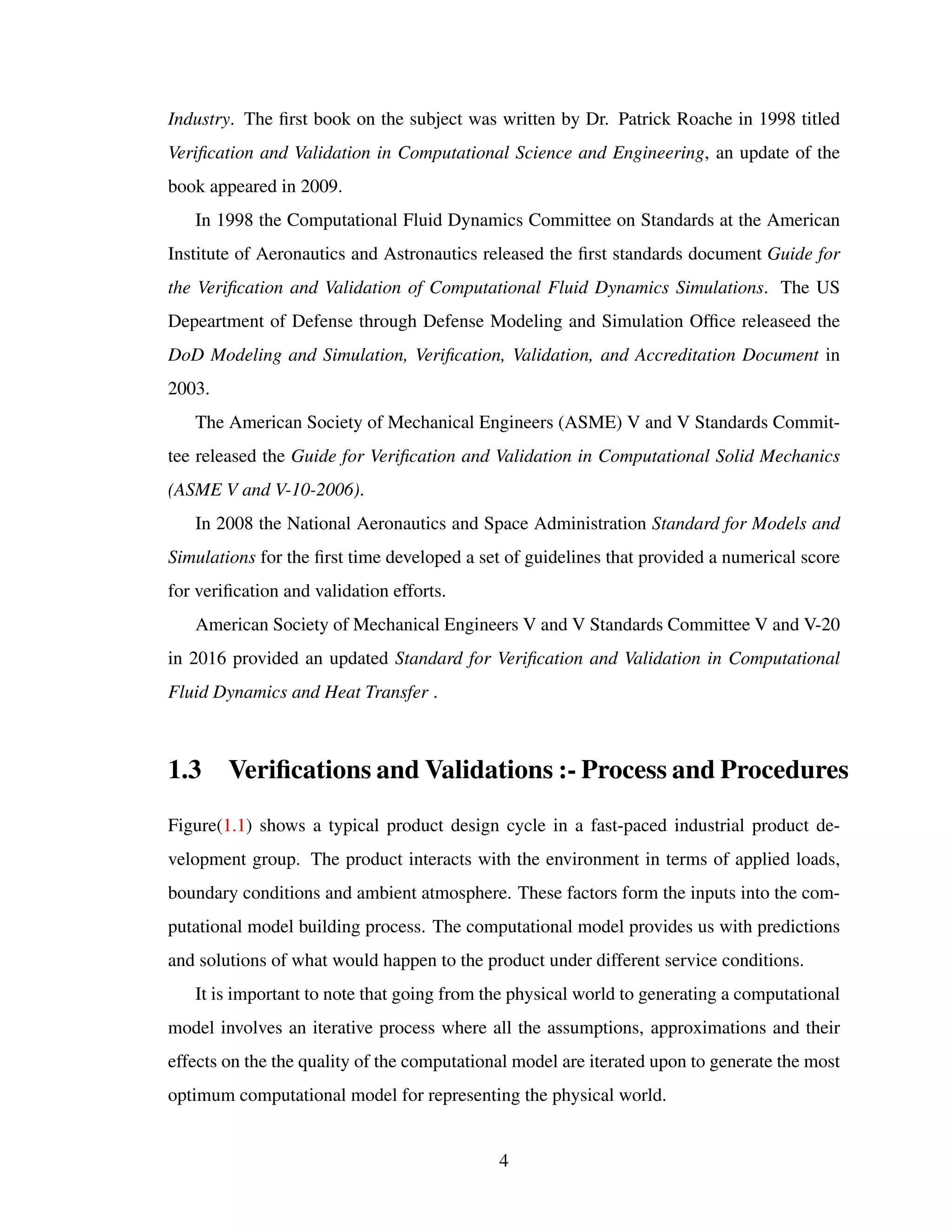
Verifications and Validations in Finite Element Analysis (FEA) using Advanced Scientific and Engineering Services AdvanSES Material characterization Fatigue Testing Strain Gauging Engineering Services Ansys Abaqus LS-Dyna MSC-Marc

1. Verifications and Validations in Finite Element
Analysis (FEA)
by
Kartik Srinivas
Advanced Scientific and Engineering Services (AdvanSES)
(An Independent Material Testing Laboratory)
212, Shukan Mall, Sabarmati-Gandhinagar Highway
Motera, Sabarmati, Ahmedabad 380005
E-mail: kartik.srinivas@advanses.com Phone: +91-9624447567
http://www.advanses.com

2. To,

3. Contents
1 Verifications and Validations in Finite Element Analysis (FEA) 1
1.1 Introduction . . . . . . . . . . . . . . . . . . . . . . . . . . . . . . . . . . 1
1.2 Brief History of Standards and Guidelines for Verifications and Validations 3
1.3 Verifications and Validations :- Process and Procedures . . . . . . . . . . . 4
1.4 Guidelines for Verifications and Validations . . . . . . . . . . . . . . . . . 8
1.5 Verification & Validation in FEA . . . . . . . . . . . . . . . . . . . . . . . 9
1.5.1 Verification Process of an FEA Model . . . . . . . . . . . . . . . . 9
1.5.2 Validation Process of an FEA Model . . . . . . . . . . . . . . . . . 12
1.6 Summary . . . . . . . . . . . . . . . . . . . . . . . . . . . . . . . . . . . 15
1.7 References . . . . . . . . . . . . . . . . . . . . . . . . . . . . . . . . . . . 16
ii

4. Verifications and Validations in Finite
Element Analysis (FEA)
1.1 Introduction
The finite element method (FEM) is a numerical method used to solve a mathematical
model of a given structure or system, which are very complex and for which analytical
solution techniques are generally not possible, the solution can be found using the finite
element method. The finite element method can thus be said to be a variational formulation
method using the principle of minimum potential energy where the unknown quantities of
interests are approximated by continuous piecewise polynomial functions. These quantities
of interest can be different according to the chosen system, as the finite element method
can be and is used in various different fields such as structural mechanics, fluid mechanics,
accoustics, electromagnetics, etc. In the field of structural mechanics the primary field of
interest is the displacements and stresses in the system.
It is important to understand that FEM only gives an approximate solution of the prob-
lem and is a numerical approach to get the real result of the variational formulation of
partial differential equations. A finite element based numerical approach gives itself to a
number of assumptions and uncertainties related to domain discretizations, mathematical
shape functions, solution procedures, etc. The widespread use of FEM as a primary tool
has led to a product engineering lifecycle where each step from ideation, design develop-
ment, to product optimization is done virtually and in some cases to the absence of even
1

5. prototype testing.
This fully virtual product development and analysis methodology leads to a situation
where a misinterpreted approximation or error in applying a load condition may be car-
ried out through out the engineering lifecycle leading to a situation where the errors get
cumulative at each stage leading to disastrous results. Errors and uncertainties in the ap-
plication of finite element method (FEM) can come from the following main sources, 1)
Errors that come from the inherent assumptions in the Finite element theory and 2) Errors
and uncertainties that get built into the system when the physics we are seeking to model
get transferred to the computational model. A common list of these kind of errors and
uncertainties are as mentioned below;
• Errors and uncertainties from the solver.
• Level of mesh refinement and the choice of element type.
• Averaging and calculation of stresses and strains from the primary solution variables.
• Uncertainty in recreating the geometrical domain on a computer.
• Approximations in the material properties of the model.
• Approximations and uncertainties in the loading and boundary conditions of the
model.
• Errors coming from chosing the right solver types for problems, e.g. Solvers for
eigen value problems.
The long list of error sources and uncertainties in the procedure makes it desirable that
a framework of rules and criteria are developed by the application of which we can make
sure that the finite element method performs within the required parameters of accuracy,
reliability and repeatability. These framework of rules serve as verification and validation
procedures by which we can consistently gauge the accuracy of our models, and sources of
errors and uncertainties be clearly identified and progressively improved to achieve greater
accuracy in the solutions. Verifications and Validations are required in each and every
2

6. development and problem solving FEA project to provide the confidence that the compu-
tational model developed performs within the required parameters. The solutions provided
by the model are sufficiently accurate and the model solves the intended problem it was
developed for.
Verification procedure includes checking the design, the software code and also inves-
tigate if the computational model accurately represents the physical system. Validation is
more of a dynamic procedure and determines if the computational simulation agrees with
the physical phenomenon, it examines the difference between the numerical simulation
and the experimental results. Verification provides information whether the computational
model is solved correctly and accurately, while validation provides evidence regarding the
extent to which the mathematical model accurately corelates to experimental tests.
In addition to complicated discretization functions, partial differential equations repre-
senting physical systema, CFD and FEA both use complicated matrices and PDE solution
algorithms to solve physical systems. This makes it imperative to carry out verification
and validation activities separately and incrementally during the model building to ensure
reliable processes. In order to avoid spurious results and data contamination giving out
false signals, it is important that the verification process is carried out before the valida-
tion assessment. If the verification process fails the the model building process should be
discontinued further until the verification is established. If the verification process suc-
ceeds, the validation process can be carried further for comparison with field service and
experimental tests.
1.2 Brief History of Standards and Guidelines for Verifi-
cations and Validations
Finite element analysis found widespread use with the release of NASA Structural Anal-
ysis Code in its various versions and flavous. The early adopters for FEA came from the
aerospace and nuclear engineering background. The first guidelines for verification and
validation were issued by the American Nuclear Society in 1987 as Guidelines for the Ver-
ification and Validation of Scientific and Engineering Computer Programs for the Nuclear
3

7. Industry. The first book on the subject was written by Dr. Patrick Roache in 1998 titled
Verification and Validation in Computational Science and Engineering, an update of the
book appeared in 2009.
In 1998 the Computational Fluid Dynamics Committee on Standards at the American
Institute of Aeronautics and Astronautics released the first standards document Guide for
the Verification and Validation of Computational Fluid Dynamics Simulations. The US
Depeartment of Defense through Defense Modeling and Simulation Office releaseed the
DoD Modeling and Simulation, Verification, Validation, and Accreditation Document in
2003.
The American Society of Mechanical Engineers (ASME) V and V Standards Commit-
tee released the Guide for Verification and Validation in Computational Solid Mechanics
(ASME V and V-10-2006).
In 2008 the National Aeronautics and Space Administration Standard for Models and
Simulations for the first time developed a set of guidelines that provided a numerical score
for verification and validation efforts.
American Society of Mechanical Engineers V and V Standards Committee V and V-20
in 2016 provided an updated Standard for Verification and Validation in Computational
Fluid Dynamics and Heat Transfer .
1.3 Verifications and Validations :- Process and Procedures
Figure(1.1) shows a typical product design cycle in a fast-paced industrial product de-
velopment group. The product interacts with the environment in terms of applied loads,
boundary conditions and ambient atmosphere. These factors form the inputs into the com-
putational model building process. The computational model provides us with predictions
and solutions of what would happen to the product under different service conditions.
It is important to note that going from the physical world to generating a computational
model involves an iterative process where all the assumptions, approximations and their
effects on the the quality of the computational model are iterated upon to generate the most
optimum computational model for representing the physical world.
4

8. Figure 1.1: Variation on the Sargent Circle Showing the Verification and Validation Pro-
cedures in a Typical Fast Paced Design Group
The validation process between the computational model and the physical world also
involves an iterative process, where experiments with values of loads and boundary con-
ditions are solved and the solution is compared to output from the physical world. The
computational model is refined based upon the feedbacks obtained during the procedure.
The circular shapes of the process representation emphasizes that computational mod-
eling and in particular verification and validation procedures are iterative in nature and
require a continual effort to optimize them.
The blue, red and green colored areas in Figure(1.3) highlight the iterative validation
and verification activities in the process. The standards and industrial guidelines clearly
mention the distinctive nature of code and solution verifications and validations at different
levels. The green highlighted region falls in the domain of the laboratory performing the
experiments, it is equally important that the testing laboratory understands both the process
and procedure of verification and validation perfectly.
Code verification seeks to ensure that there are no programming mistakes or bugs and
that the software provides the accuracy in terms of the implementation of the numerical al-
gorithms or construction of the solver. Comparing the issue of code verification and calcu-
lation verification of softwares, the main point of difference is that calculation verification
5

9. Figure 1.2: Verification and Validation Process
involves quantifying the discretization error in a numerical simulation. Code verification is
rather upstream in the process and is done by comparing numerical results with analytical
solutions.
6

10. Figure 1.3: Guidance for Verification and Validation as per ASME 10.1 Standard
7

11. 1.4 Guidelines for Verifications and Validations
The first step is the verification of the code or software to confirm that the software is work-
ing as it was intended to do. The idea behind code verification is to identify and remove
any bugs that might have been generated while implementing the numerical algorithms or
because of any programming errors. Code verification is primarily a responsibility of the
code developer and softwares like Abaqus, LS-Dyna etc., provide example problems man-
uals, benchmark manuals to show the verifications of the procedures and algorithms they
have implemented.
Next step of calculation verification is carried out to quantify the error in a computer
simulation due to factors like mesh discretization, improper convergence criteria, approxi-
mation in material properties and model generations. Calculation verification provides with
an estimation of the error in the solution because of the mentioned factors. Experience has
shown us that insufficient mesh discretization is the primary culprit and largest contributor
to errors in calculation verification.
Validation processes for material models, elements, and numerical algorithms are gen-
erally part of FEA and CFD software help manuals. However, when it comes to estab-
lishing the validity of the computational model that one is seeking to solve, the validation
procedure has to be developed by the analyst or the engineering group.
The following validation guidelines were developed at Sandia National Labs[Oberkampf
et al.] by experimentalists working on wind tunnel programs, however these are applicable
to all problems from computational mechanics.
Guideline 1: The validation experiment should be jointly designed by the FEA group
and the experimental engineers. The experiments should ideally be designed so that the
validation domain falls inside the application domain.
Guideline 2: The designed experiment should involve the full physics of the system,
including the loading and boundary conditions.
Guideline 3: The solutions of the experiments and from the computational model
should be totally independent of each other.
Guideline 4: The experiments and the validation process should start from the system
8

12. level solution to the component level.
Guideline 5: Care should be taken that operator bias or process bias does not contami-
nate the solution or the validation process.
1.5 Verification & Validation in FEA
1.5.1 Verification Process of an FEA Model
In the case of automotive product development problems, verification of components like
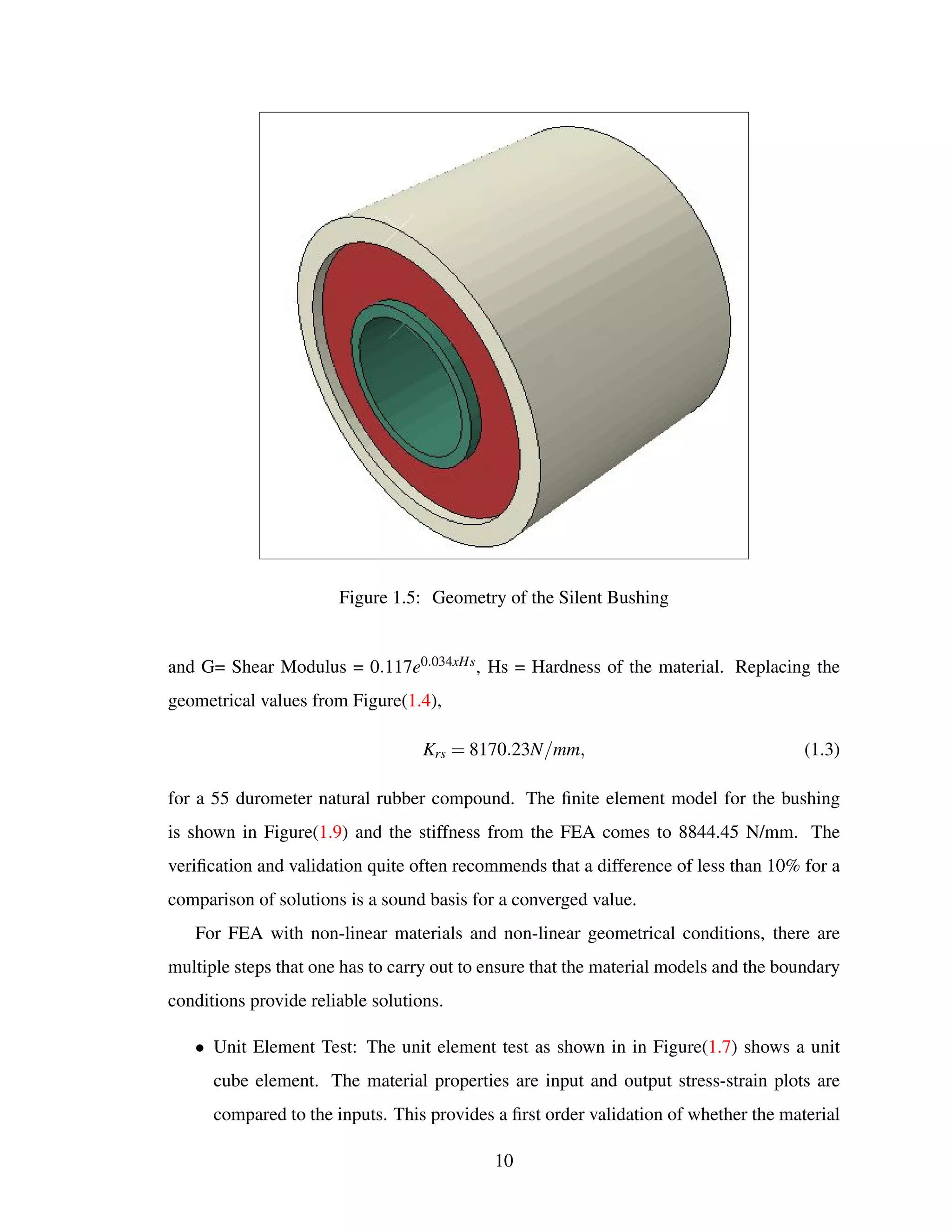
silent blocks and bushings, torque rod bushes, spherical bearings etc., can be carried. Fig-
ure(1.4) shows the rubber-metal bonded component for which calculations have been car-
ried out. Hill[11], Horton[12] and have shown that under radial loads the stiffness of the
bushing can be given by,
Figure 1.4: Geometry Dimensions of the Silent Bushing
Krs = βrsLG (1.1)
where,βrs =
80π A2 +B2
25(A2 +B2)ln B
A −9(A2 −B2)
(1.2)
9

13. Figure 1.5: Geometry of the Silent Bushing
and G= Shear Modulus = 0.117e0.034xHs, Hs = Hardness of the material. Replacing the
geometrical values from Figure(1.4),
Krs = 8170.23N/mm, (1.3)
for a 55 durometer natural rubber compound. The finite element model for the bushing
is shown in Figure(1.9) and the stiffness from the FEA comes to 8844.45 N/mm. The
verification and validation quite often recommends that a difference of less than 10% for a
comparison of solutions is a sound basis for a converged value.
For FEA with non-linear materials and non-linear geometrical conditions, there are
multiple steps that one has to carry out to ensure that the material models and the boundary
conditions provide reliable solutions.
• Unit Element Test: The unit element test as shown in in Figure(1.7) shows a unit
cube element. The material properties are input and output stress-strain plots are
compared to the inputs. This provides a first order validation of whether the material
10

14. Figure 1.6: Deformed Shape of the Silent Bushing
properties are good enough to provide sensible outputs. The analyst him/her self can
carry out this validation procedure.
• Experimental Characterization Test: FEA is now carried out on a characterization test
such as a tension test or a compression test. This provides a checkpoint of whether
the original input material data can be backed out from the FEA. This is a moderately
difficult test as shown in Figure(1.8). The reasons for the difficulties are because of
unquantified properties like friction and non-exact boundary conditions.
• Comparison to Full Scale Experiments: In these validation steps, the parts and com-
ponent products are loaded up on a testing rig and service loads and boundary con-
ditions are applied. The FEA results are compared to these experiments. This step
provides the most robust validation results as the procedure validates the finite ele-
ment model as well as the loading state and boundary conditions. Figure(1.9) shows
torque rod bushing and the validation procedure carried out in a multi-step analysis.
Experience shows that it is best to go linearly in the validation procedure from step 1
11

15. through 3, as it progressively refines one’s material model, loading, boundary conditions.
Directly jumping to step 3 to complete the validation process faster adds upto more time
with errors remaining unresolved, and these errors go on to have a cumulative effect on the
quality of the solutions.
Figure 1.7: Unit Cube Single Element Test
Figure 1.8: FEA of Compression Test
1.5.2 Validation Process of an FEA Model
Figure(1.7) shows the experimental test setup for validation of the bushing model. Radial
loading is chosen to be the primary deformation mode and load vs. displacement results
are compared. The verification process earlier carried out established the veracity of the
FEA model and the current validation analysis applies the loading in multiple Kilonewtons.
Results show a close match between the experimental and FEA results. Figures(1.10) and
12

16. Figure 1.9: Experimental Testing and Validation FEA for the Silent Bushing
(1.11) show the validation setup and solutions for a tire model and engine mount. The
complexity of a tire simulation is due to the nature of the tire geometry, and the presence
of multiple rubber compounds, fabric and steel belts. This makes it imperative to establish
the validity of the simulations.
13

17. Figure 1.10: Experimental Testing and Validation FEA for a Tire Model
Figure 1.11: Experimental Testing and Validation FEA for a Passenger Car Engine Mount
14

18. 1.6 Summary
An attempt was made in the article to provide information on the verification and validation
processes in computational solid mechanics. We went through the history of adoption
of verification and validation processes and their integration in computational mechanics
processes and tools. Starting from 1987 when the first guidelines were issued in a specific
field of application, today we are at a stage where the processes have been standardized and
all major industries have found their path of adoption.
Verification and validations are now an integral part of computational mechanics pro-
cesses to increase integrity and reliability of the solutions. Verification is done primarily at
the software level and is aimed at evaluating whether the code has the capability to offer the
correct solution to the problem, while validation establishes the accuracy of the solution.
ASME, Nuclear Society and NAFEMS are trying to make the process more standardized,
and purpose driven.
Uncertainty quantification has not included in this current review, the next update of
this article will include steps for uncertainty quantification in the analysis.
15

19. 1.7 References
1. American Nuclear Society, Guidelines for the Verification and Validation of Scientific
and Engineering Computer Programs for the Nuclear Industry 1987.
2. Roache, P.J, American Nuclear Society, Verification and Validation in Computational
Science and Engineering, Hermosa Publishing, 1998.
3. American Institute of Aeronautics and Astronautics, AIAA Guide for the Verification
and Validation of Computational Fluid Dynamics Simulations (G-077-1998), 1998.
4. U.S. Department of Defense, DoD Modeling and Simulation (M-S) Verification, Val-
idation, and Accreditation, Defense Modeling and Simulation Office, Washington,
DC.
5. American Society of Mechanical Engineers, Guide for Verification and Validation in
Computational Solid Mechanics, 2006.
6. Thacker, B. H., Doebling S. W., Anderson M. C., Pepin J. E., Rodrigues E. A.,
Concepts of Model Verification and Validation, Los Alamos National Laboratory,
2004.
7. Standard for Models And Simulations, National Aeronautics and Space Administra-
tion, NASA-STD-7009, 2008.
8. Oberkampf, W.L. and Roy, C.J., Verification and Validation in Computational Simu-
lation, Cambridge University Press, 2009.
9. Austrell, P. E., Olsson, A. K. and Jonsson, M. 2001, A Method to analyse the non-
Linear dynamic behaviour of rubber components using standard FE codes, Paper no
464. Conference on Fluid and Solid Mechanics.
10. Austrell, P. E., Modeling of Elasticity and Damping for Filled Elastomers,Lund Uni-
versity.
11. ABAQUS Inc., ABAQUS: Theory and Reference Manuals, ABAQUS Inc., RI, 02.
16

20. 12. Hill, J. M. Radical deflections of rubber bush mountings of finite lengths. Int. J. Eng.
Sci., 1975, 13.
13. Horton, J. M., Gover, M. J. C. and Tupholme, G. E. Stiffness of rubber bush mount-
ings subjected to radial loading. Rubber Chem. Tech., 2000, 73.
14. Lindley, P. B. Engineering design with natural rubber , The Malaysian Rubber Pro-
ducers’ Research Association, Brickendonbury, UK., 1992.
15. Attard, M.M., Finite Strain: Isotropic Hyperelasticity, International Journal of Solids
and Structures, 2003.
16. Srinivas, K., Pannikottu, A., Gerhardt, J., Material Characterization Testing and Fi-
nite Element Analysis of a SUV Tire for Prediction of Performance, India Rubber
Expo, 2005.
17. Srinivas, K., and Dharaiya, D., Material And Rheological Characterization For Rapid
Prototyping Of Elastomers Components, American Chemical Society, Rubber Divi-
sion, 170th Technical Meeting, Cincinnati, 2006.
18. Bathe, K. J., Finite Element Procedures Prentice-Hall, NJ, 96.
19. Bergstrom, J. S., and Boyce, M. C., Mechanical Behavior of Particle Filled Elas-
tomers, Rubber Chemistry and Technology, Vol. 72, 2000.
20. Beatty, M.F., Topics in Finite Elasticity: Hyperelasticity of Rubber, Elastomers and
Biological Tissues with Examples, Applied Mechanics Review, Vol. 40, No. 12,
1987.
21. Erdemir, A., Guess, T. M., Halloran, J., STadepalli, S. C., Morrison, T. M., Consid-
erations for Reporting Finite Element Analysis Studies in Biomechanics, J Biomech.
2012 February 23; 45(4).
22. Blatz, P. J., Application of Finite Elasticity Theory to the Behavior of Rubberlike
Materials, Transactions of the Society of Rheology, Vol. 6, 1962.
17

21. 23. Boyce, M. C., and Arruda, E. M., Constitutive Models of Rubber Elasticity: A Re-
view, Rubber Chemistry and Technology, Vol. 73, 2000.
24. Callister Jr., W. D., Introduction to Materials Science and Engineering John Wiley
and Sons, NY, 1999.
25. Cescotto, S., and Fonder, G., A Finite Element Aprroach for Large Strains of Nearly
Incompressible Rubber Like Materials, International Journal of Solids and Struc-
tures, Vol. 15, 1979.
26. Charlton, D. J., and Yang, J., A Review of Methods to Characterize Rubber Elastic
Behavior for use in Finite Element Analysis, Rubber Chemistry and Technology, Vol.
67, 1994.
27. Crisfield, M. A., Non-linear Finite Element Analysis of Solids and Structures, Vol. I,
John Wiley and Sons, NY, 2000.
28. Crisfield, M. A., Non-linear Finite Element Analysis of Solids and Structures, Vol. II,
John Wiley and Sons, NY, 2000.
29. Tina M. Morrison, Maureen L. Dreher, Srinidhi Nagaraja, Leonardo M. Angelone,
Wolfgang Kainz, The Role of Computational Modeling and Simulation in the Total
Product Life Cycle of Peripheral Vascular Devices, J of Med Device. 2017 ; 11(2).
30. Daley, J. R. and Mays, S., The Complexity of Material Modeling in the Design Opti-
mization of Elastomeric Seals, Finite Element Analysis of Elastomers, Professional
Engineering Publishing, London, 1999.
31. Dowling, N. E., Mechanical Behavior of Materials, Engineering Methods for Defor-
mation, Fracture and Fatigue Prentice-Hall, NJ, 99.
32. Du Bois, P. A., A Simplified Approach to the Simulation of Rubber-like Materials
Under Dynamic Loading, 4th European LS-Dyna Users Conference, 2003.
18

22. 33. Jaehyeok Doh, Sang-Woo Kim, Jongsoo Lee Reliability assessment on the degrada-
tion properties of polymers under operating temperature and vibration conditions,
Journal of Automobile Engineering, October 2017.
34. Christensen, R. Theory of viscoelasticity: An introduction, Elsevier, New York, 2012.
35. Feng, W. W., and Hallquist, J. O., On Constitutive Equations for Elastomers and
Elastomeric Foams, 4th European LS-Dyna Users Conference, 2003.
36. Juan Sebastian Arrieta, Julie Diani, Pierre Gilormini Experimental characterization
and ThermoViscoelastic Modeling of Strain and Stress Recoveries of an Amorphous
Polymer Network, Mechanics of materials, Vol. 68, p.95-103 - 2014
37. Dalrymple, Todd. Answers to Questions on Simulia Social Media Account Website,
www.swym.3ds.com, 2016.
38. Finney, R. H., and Kumar, A., Development of Material Constants for Non-linear
Finite Element Analysis, Rubber Chemistry and Technology, Vol. 61, 1988.
39. Gent, N. A.,Engineering with Rubber: How to Design Rubber Components, Hanser
Publishers, NY, 92.
40. Gent, N. A.,A New Constitutive Relation for Rubber, Rubber Chemistry and Tech-
nology, Vol. 69, 1996.
41. Goran, S., Stress Relaxation Tests, Elastocon AB Technical Report, 1999.
42. Heinbockel, J. H., Introduction to Tensor Calculus and Continuum Mechanics, Traf-
ford Publishing, http://www.math.odu.edu/ jhh
43. Hertz, D. L. Jr., Designing with Elastomers, Seals Eastern, Inc. 1983.
44. Ionita Axinte, Finite Element Analysis of the Deformation of a Rubber Diaphragm,
P.hD Dissertation, Virginia Polytechnic and State University, 2001.
45. LSTC, LS-DYNA Users Manual, Version 960, Livermore Software Technology Cor-
poration, March 2001.
19

23. 46. Makino, A., Hamburgen, W. R., and Fitch, J. S., Fluoroelastomer Pressure Pad De-
sign for Microelectronic Applications, DEC Western Research Laboratory, WRL-
93/7, 1993.
47. Minnesota Rubber, Elastomers and Thermoplastics Engineering Design Guide, Min-
nesota Rubber and QMR Plastics, 2003.
48. MSC Software, MSC MARC Reference Manuals, MSC Software, CA 02.
49. Lobo, H., Providing an Experimental Basis in Support of FEA, Simulia Customer
Conference, 2014.
50. Megan, L. and Brian Croop, A Mechanism for the Validation of Hyperelastic Mate-
rials in ANSYS, Datapointlabs.
51. Mullins, L. Softening of Rubber by Deformation Rubber Chemistry and Technology,
Vol.42, 1969.
52. Nicholson, D. W., and Nelson, N. W., Finite Element Analysis in Design with Rubber,
Rubber Chemistry and Technology, Vol. 63, 1990.
53. Srinivas, K., Systematic Experimental and Computational Mechanics Analysis Method-
ologies for Polymer Components, ARDL Technical Report, March 2008.
54. Schwer, L. E., Verification and Validation in Computational Solid Mechanics and the
ASME Standards Committee, WIT Transactions on The Built Environment, Vol. 84,
2005.
55. Oberkampf, W. L., Trucano, T. G., and Hirsch, C., Verification, Validation and Pre-
dictive Capability in Computational Engineering and Physics, Foundations for Veri-
fication and Validation in the 21st Century Workshop, 2002.
56. Ogden, R. W. Non-linear Elastic Deformations, Dover Publications, NY, 1997.
20