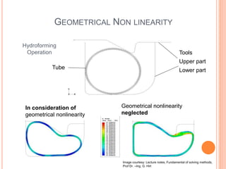
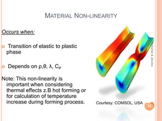
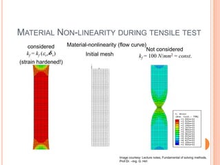
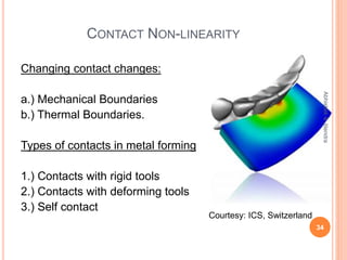
Contact: abhishek.hukkerikar@rwth-aachen.de
WHAT IS ANALYSIS?
2
Abhishek&Jitendra
"In 1 million to 10 million years they
might be able to make a plane that
would fly."
-The New York Times, 1903
Imagination
ModelApplication
200 meters384,400 kilometers
METHODS OF ANALYSES
Mode of
analyses
Analytical &
numerical methods
Elementary theory
Slip Line
field theory
Finite
Element
Method
(FEM)
Finite Difference
method (FDM)
Upper &
Lower Bound
method
Empirical
Methods
Similarity theory
Visio plastic
method
3
Abhishek&Jitendra
Image courtesy: Lecture notes, Fundamental of solving methods,
Prof Dr. –Ing. G. Hirt
ELEMENTARY PLASTICITY THEORY
Approach:
Establishment of kinetics relative to
the process.
Establishment of differential
equations suiting the process &
the simplification.
4
Abhishek&Jitendra
UPPER & LOWER BOUNDARY METHOD
Method approximates the values of deforming forces to be
higher or lower than actual forces.
“Any estimate of the collapse load of a structure made by
equating the rate of the energy dissipation internally to the
rate at which external forces do work, in some assumed
pattern of the deformation will be greater than or equal to
the correct load”
-W.F. Hosford & R.M Caddell
Assumptions of the method:
 Material being deformed is isotropic & homogenous
 There is no effect of work hardening
 No friction exists between work piece & tool interface.
 Plane strain conditions assumed.
5
Abhishek&Jitendra
William Hosford
due to
frictionless
upsetting
due to
Symmetr
y
Symmetr
y plane
Slip
line on
the
edge
SLIP-LINE THEORY
Here flow pattern from point to point while
deformation is considered & analyzed.
Slip line refers to the planes of maximum shear
stress which are inclined at 45o to the principle
planes.
Assumptions of the method:
 Material being deformed is isotropic &
homogenous
 There is no effect of work hardening & strain rate.
 No friction exists between work piece & tool
interface.
 Plane strain conditions assumed.
 Effect of temperature , strain rate, & time
neglected.
6
Abhishek&Jitendra
Image courtesy: Lecture notes, Fundamental of solving methods,
Prof Dr. –Ing. G. Hirt
COMPARISON
FEM
• Material flow analysis &
local states of stress &
strain described.
• Various boundary
conditions can be applied.
• Multi-axial stress in
consideration
Analytical methods
• Only Global analysis is done.
• Material homogeneity is assumed.
• 2-deminsional conditions.
• Temperature effects neglected.
7
Abhishek&Jitendra
FINITE ELEMENT ANALYSIS
A brief history
 Concept was developed by the works of Richard
Courant & Alexander Hrennikoff (early 40’s).
 Idea was originated to solve complex problems
of civil engineering & structural analysis.
 Idea was promoted by Boeing to compute sweep
of airplane wings (mid 50’s).
 M.J Turner & Ray W. Clough articles established
the applications of FEA (mid 50’s).
 Idea was also used to compute roof of Munich
Olympic stadium (late 60’s) 8
Abhishek&Jitendra
Richard Courant
R.W.Clough
AREAS OF APPLICATIONS
9
Abhishek&Jitendra
Engineering
• Fluid mechanics
• Thermodynamics
• Metal Forming etc
Biological Sciences
• Botany
• Zoology
• Archeological Anthropology
• Paleontology
General application
• Geology
• Astrophysics
ENGINEERING APPLICATIONS
10
Abhishek & Jitendra
C-blade Forging &
Manufacturing
Department of electronics &
Telecommunications, University of
Naples,Italy
Hochschule Regensburg,
Biomechanik
Numerical assessment of static & seismic behavior of
the Basilica of Santa Maria all’Impruneta (Italy)
Department of Atomic & Solid state
physics University of Cornell
Lehrstuhl Numerische Mathematik,
Ruprecht-Karls-Universität, Heidelberg
HIERARCHY OF FEM
Physical Problem
Establish Finite element
model of the physical problem
Solve the problem
Interpret the result 11
Abhishek&Jitendra
SPACE INCREMENTATION
Finite Elements:
 Every model is sub-divided into
finite elements. Their junction
points are called as nodes.
 Model assumes that forces act at
nodes & stresses & strain exist at
the finite element.
 Reliability of FEA depends on
number of finite elements.
12
Abhishek&Jitendra
STIFFNESS MATRIX
 
FuK
L
AE






















2
1
2
1
F
F
u
u
11
11
  
)( 121 uu
L
AE
F 







































3
2
1
3
2
1
110
121
011
F
F
F
u
u
u
L
AE
13
Example: Beams protruding from fixed surface
u
u
2
u1
F1 F2
Stiffness Coeffecient Force
)( 212 uu
L
AE
F 


Displacement
Stiffness Matrix
SPACE INCREMENTATION
Element types:
14
Abhishek&Jitendra
Image courtesy: Lecture notes, Fundamental of solving methods,
Prof Dr. –Ing. G. Hirt
SPACE INCREMENTATION
Meshing
Network of nodes is called a mesh.
There are 2 broad mesh-generation
methods.
 Unstructured( Formed
automatically) A
 Structured (Formed by grid based
sub-dividing of geometry) B 15
Abhishek&Jitendra
SPACE INCREMENTATION
Meshing:
 Accuracy of results always
depends on the assumptions.
 Fine mesh is considered where
there are stress & strain
gradients.
 A coarse mesh is used in the
areas of reasonably constant
stress or areas of interest.
16
Abhishek&Jitendra
PROTOCOLS
 Gaps are not permitted
during meshing.
 Nodes are numbered
sequentially.
17
Abhishek&Jitendra
SPACE INCREMENTATION
Approaches:
LAGRANGE’S approach
 Mesh is bound to the material
 Mesh will be distorted with
increasing deformation.
18
Abhishek&Jitendra
Courtesy: FHWA. USA
SPACE INCREMENTATION
EULER’S Approach
 Mesh is fixed & not bound
to the material.
 Material flows through
fixed mesh.
19
Abhishek&Jitendra
SPACE INCREMENTATION
Remeshing
Why is it necessary?
 Formation of unacceptable shapes due to large local deformations.
 High relative motion between die surface & deforming material.
 Large displacement causes computational problems.
 Difficulties encountered in incorporating die boundary shapes with
increase in relative displacement.
To overcome above difficulties, periodic redefining of mesh is necessary 21
Abhishek&Jitendra
SPACE INCREMENTATION
Remeshing comprises of following
steps:
1. Assignment of new mesh
system to work piece
2. Transfer of information (strain,
strain rate, & temperature)
from the old to the new mesh
through interpolation.
22
Abhishek&Jitendra
Image courtesy: emerald.com
SOLVERS
For simulation of metal forming, following 2 solutions
are used:
 Implicit method ( Stable, iterative, high
computational effort)
 Explicit method (conditionally stable, no iteration,
less computational effort)
23
Abhishek&Jitendra
IMPLICIT SOLVERS
 Studies reveal that this solver is
useful in smaller & 2D problems.
 Each time step or increment has
to be treated as unconditionally
stable process.
 Large time steps lead to larger
iterations & process do not
converge.
24
Abhishek&Jitendra
(Newton Raphson method )Non-
linear analysis of reinforced
concrete beam
IMPLICIT SOLVERS
In the implicit approach a solution to the set of finite
element equations involves iteration until a convergence
criterion is satisfied for each increment.
 Here computation is divided into several calculation time
steps.
 At the end of each time step(increment) the equilibrium
between internal & external load must be reached.
 Else iteration continues.
25
Abhishek&Jitendra
EXPLICIT SOLVERS
 The finite element equations in the explicit approach are
reformulated as being dynamic.
 In this form they can be solved directly to determine the
solution at the end of the increment, without iteration.
 Two methods are followed for time step calculations.
26
Abhishek&Jitendra
EXPLICIT SOLVERS
Here largest allowable time step for a stable solution depends on:
 Highest Eigen frequency occurring (ωmax )in the system
 Corresponding damping (ξ)
∆tm ≤ (2/ωmax)* ((1+ξ2)0.5-ξ)
Sonic frequency & smallest element Le are estimated as follows:
∆ t ≤Le /C with C=(E/ρ)0.5
To compensate the disadvantage of extremely small time step, will
be reduced through increasing the density or shortening the process
time.
27
Abhishek&Jitendra
COMPUTATIONAL TIME REQUIRED FOR
EXPLICIT/IMPLICIT METHODS
implicit: Complexity ~ number of freedom degrees x wave front
explicit: Complexity ~ number of freedom degrees
Complexity
Implicit
Explicit
Model-size
(Calculation time)
Efficiency
Statics Structural
dynamics
Highly
dynamic
Implicit Explicit
Image courtesy: Lecture notes, Fundamental of solving methods,
Prof Dr. –Ing. G. Hirt
NON-LINEARITIES IN FEM
Following Non-linearities are encountered during the
simulations.
 Geometrical Non-linearity
 Material Non-linearity
 Contact variance (Change of boundary conditions)
 Friction
29
Abhishek&Jitendra
GEOMETRICAL NON-LINEARITY
In practical cases it is not
uncommon to encounter
strain of magnitude 2 or more
due to :
 Large elongation
 Large rotation
 Portions of rigid body
movements 30
Abhishek&Jitendra
Courtesy: MRF tyres, India
GEOMETRICAL NON LINEARITY
Hydroforming
Operation Tools
Upper part
Lower partTube
In consideration of
geometrical nonlinearity
Geometrical nonlinearity
neglected
Image courtesy: Lecture notes, Fundamental of solving methods,
Prof Dr. –Ing. G. Hirt
MATERIAL NON-LINEARITY
Occurs when:
 Transition of elastic to plastic
phase
 Depends on ρ,θ, λ, CP
Note: This non-linearity is
important when considering
thermal effects z.B hot forming or
for calculation of temperature
increase during forming process.
32
Abhishek&Jitendra
Courtesy: COMSOL, USA
Material-nonlinearity (flow curve)
MATERIAL NON-LINEARITY DURING TENSILE TEST
Image courtesy: Lecture notes, Fundamental of solving methods,
Prof Dr. –Ing. G. Hirt
kf = kf (v, v)
(strain hardened!)

considered Not considered
kf = 100 N/mm2 = const.Initial mesh
CONTACT NON-LINEARITY
Changing contact changes:
a.) Mechanical Boundaries
b.) Thermal Boundaries.
Types of contacts in metal forming
1.) Contacts with rigid tools
2.) Contacts with deforming tools
3.) Self contact
34
Abhishek&Jitendra
Courtesy: ICS, Switzerland
FRICTION
Friction is non-linear. Friction leads to asymmetrical
equation system. This increases the calculation
complexity.
Categorization:
1. τ<µσN -- Sticking friction
2. τ=µσN – Slide friction
35
Abhishek&Jitendra
WHY IS FEM ADVANTAGEOUS OVER OTHER
SOLVING METHODS
36
Abhishek&Jitendra
without friction
with friction
Upsetting
without friction with friction
Comparision with & without
friction during upsetting
Image courtesy: Lecture notes, Fundamental of solving methods,
Prof Dr. –Ing. G. Hirt
VOTE OF THANKS & REFERENCES
Sincerely indebted to:
Prof Dr. –Ing. G. Hirt, Head of the department, IBF, RWTH Aachen
Dipl.-Ing. Simon Seuren, IBF, RWTH Aachen
Institute of Metal Forming, RWTH Aahcen
References:
 Fundamentals of solving methods in metal forming by Prof.Dr.- Ing.G.Hirt
 Metal forming & finite element method –Atlan,Oh, Kobayashi
 Manufacturing process III –A.C.Niranjan
 Comparison of the implicit and explicit finite element methods
using crystal plasticity- F.J. Harewood , P.E. McHugh
Web resources:
 National program on technology enhanced learning, Dr. R. Krishnakumar, IIT madras.
38
Abhishek&Jitendra
THANK YOU FOR YOUR PATIENCE & KIND ATTENTION!
FOR FURTHER DETAILS, QUERIES, AND SUGGESTIONS,
CONTACT US ON:
39
Abhishek&Jitendra
abhishek.hukkerikar@rwth-aachen.de

Finite Element Analysis in Metal Forming processes

  • 1.
  • 2.
    WHAT IS ANALYSIS? 2 Abhishek&Jitendra "In1 million to 10 million years they might be able to make a plane that would fly." -The New York Times, 1903 Imagination ModelApplication 200 meters384,400 kilometers
  • 3.
    METHODS OF ANALYSES Modeof analyses Analytical & numerical methods Elementary theory Slip Line field theory Finite Element Method (FEM) Finite Difference method (FDM) Upper & Lower Bound method Empirical Methods Similarity theory Visio plastic method 3 Abhishek&Jitendra Image courtesy: Lecture notes, Fundamental of solving methods, Prof Dr. –Ing. G. Hirt
  • 4.
    ELEMENTARY PLASTICITY THEORY Approach: Establishmentof kinetics relative to the process. Establishment of differential equations suiting the process & the simplification. 4 Abhishek&Jitendra
  • 5.
    UPPER & LOWERBOUNDARY METHOD Method approximates the values of deforming forces to be higher or lower than actual forces. “Any estimate of the collapse load of a structure made by equating the rate of the energy dissipation internally to the rate at which external forces do work, in some assumed pattern of the deformation will be greater than or equal to the correct load” -W.F. Hosford & R.M Caddell Assumptions of the method:  Material being deformed is isotropic & homogenous  There is no effect of work hardening  No friction exists between work piece & tool interface.  Plane strain conditions assumed. 5 Abhishek&Jitendra William Hosford
  • 6.
    due to frictionless upsetting due to Symmetr y Symmetr yplane Slip line on the edge SLIP-LINE THEORY Here flow pattern from point to point while deformation is considered & analyzed. Slip line refers to the planes of maximum shear stress which are inclined at 45o to the principle planes. Assumptions of the method:  Material being deformed is isotropic & homogenous  There is no effect of work hardening & strain rate.  No friction exists between work piece & tool interface.  Plane strain conditions assumed.  Effect of temperature , strain rate, & time neglected. 6 Abhishek&Jitendra Image courtesy: Lecture notes, Fundamental of solving methods, Prof Dr. –Ing. G. Hirt
  • 7.
    COMPARISON FEM • Material flowanalysis & local states of stress & strain described. • Various boundary conditions can be applied. • Multi-axial stress in consideration Analytical methods • Only Global analysis is done. • Material homogeneity is assumed. • 2-deminsional conditions. • Temperature effects neglected. 7 Abhishek&Jitendra
  • 8.
    FINITE ELEMENT ANALYSIS Abrief history  Concept was developed by the works of Richard Courant & Alexander Hrennikoff (early 40’s).  Idea was originated to solve complex problems of civil engineering & structural analysis.  Idea was promoted by Boeing to compute sweep of airplane wings (mid 50’s).  M.J Turner & Ray W. Clough articles established the applications of FEA (mid 50’s).  Idea was also used to compute roof of Munich Olympic stadium (late 60’s) 8 Abhishek&Jitendra Richard Courant R.W.Clough
  • 9.
    AREAS OF APPLICATIONS 9 Abhishek&Jitendra Engineering •Fluid mechanics • Thermodynamics • Metal Forming etc Biological Sciences • Botany • Zoology • Archeological Anthropology • Paleontology General application • Geology • Astrophysics
  • 10.
    ENGINEERING APPLICATIONS 10 Abhishek &Jitendra C-blade Forging & Manufacturing Department of electronics & Telecommunications, University of Naples,Italy Hochschule Regensburg, Biomechanik Numerical assessment of static & seismic behavior of the Basilica of Santa Maria all’Impruneta (Italy) Department of Atomic & Solid state physics University of Cornell Lehrstuhl Numerische Mathematik, Ruprecht-Karls-Universität, Heidelberg
  • 11.
    HIERARCHY OF FEM PhysicalProblem Establish Finite element model of the physical problem Solve the problem Interpret the result 11 Abhishek&Jitendra
  • 12.
    SPACE INCREMENTATION Finite Elements: Every model is sub-divided into finite elements. Their junction points are called as nodes.  Model assumes that forces act at nodes & stresses & strain exist at the finite element.  Reliability of FEA depends on number of finite elements. 12 Abhishek&Jitendra
  • 13.
    STIFFNESS MATRIX   FuK L AE                       2 1 2 1 F F u u 11 11   )( 121 uu L AE F                                         3 2 1 3 2 1 110 121 011 F F F u u u L AE 13 Example: Beams protruding from fixed surface u u 2 u1 F1 F2 Stiffness Coeffecient Force )( 212 uu L AE F    Displacement Stiffness Matrix
  • 14.
    SPACE INCREMENTATION Element types: 14 Abhishek&Jitendra Imagecourtesy: Lecture notes, Fundamental of solving methods, Prof Dr. –Ing. G. Hirt
  • 15.
    SPACE INCREMENTATION Meshing Network ofnodes is called a mesh. There are 2 broad mesh-generation methods.  Unstructured( Formed automatically) A  Structured (Formed by grid based sub-dividing of geometry) B 15 Abhishek&Jitendra
  • 16.
    SPACE INCREMENTATION Meshing:  Accuracyof results always depends on the assumptions.  Fine mesh is considered where there are stress & strain gradients.  A coarse mesh is used in the areas of reasonably constant stress or areas of interest. 16 Abhishek&Jitendra
  • 17.
    PROTOCOLS  Gaps arenot permitted during meshing.  Nodes are numbered sequentially. 17 Abhishek&Jitendra
  • 18.
    SPACE INCREMENTATION Approaches: LAGRANGE’S approach Mesh is bound to the material  Mesh will be distorted with increasing deformation. 18 Abhishek&Jitendra Courtesy: FHWA. USA
  • 19.
    SPACE INCREMENTATION EULER’S Approach Mesh is fixed & not bound to the material.  Material flows through fixed mesh. 19 Abhishek&Jitendra
  • 20.
    SPACE INCREMENTATION Remeshing Why isit necessary?  Formation of unacceptable shapes due to large local deformations.  High relative motion between die surface & deforming material.  Large displacement causes computational problems.  Difficulties encountered in incorporating die boundary shapes with increase in relative displacement. To overcome above difficulties, periodic redefining of mesh is necessary 21 Abhishek&Jitendra
  • 21.
    SPACE INCREMENTATION Remeshing comprisesof following steps: 1. Assignment of new mesh system to work piece 2. Transfer of information (strain, strain rate, & temperature) from the old to the new mesh through interpolation. 22 Abhishek&Jitendra Image courtesy: emerald.com
  • 22.
    SOLVERS For simulation ofmetal forming, following 2 solutions are used:  Implicit method ( Stable, iterative, high computational effort)  Explicit method (conditionally stable, no iteration, less computational effort) 23 Abhishek&Jitendra
  • 23.
    IMPLICIT SOLVERS  Studiesreveal that this solver is useful in smaller & 2D problems.  Each time step or increment has to be treated as unconditionally stable process.  Large time steps lead to larger iterations & process do not converge. 24 Abhishek&Jitendra (Newton Raphson method )Non- linear analysis of reinforced concrete beam
  • 24.
    IMPLICIT SOLVERS In theimplicit approach a solution to the set of finite element equations involves iteration until a convergence criterion is satisfied for each increment.  Here computation is divided into several calculation time steps.  At the end of each time step(increment) the equilibrium between internal & external load must be reached.  Else iteration continues. 25 Abhishek&Jitendra
  • 25.
    EXPLICIT SOLVERS  Thefinite element equations in the explicit approach are reformulated as being dynamic.  In this form they can be solved directly to determine the solution at the end of the increment, without iteration.  Two methods are followed for time step calculations. 26 Abhishek&Jitendra
  • 26.
    EXPLICIT SOLVERS Here largestallowable time step for a stable solution depends on:  Highest Eigen frequency occurring (ωmax )in the system  Corresponding damping (ξ) ∆tm ≤ (2/ωmax)* ((1+ξ2)0.5-ξ) Sonic frequency & smallest element Le are estimated as follows: ∆ t ≤Le /C with C=(E/ρ)0.5 To compensate the disadvantage of extremely small time step, will be reduced through increasing the density or shortening the process time. 27 Abhishek&Jitendra
  • 27.
    COMPUTATIONAL TIME REQUIREDFOR EXPLICIT/IMPLICIT METHODS implicit: Complexity ~ number of freedom degrees x wave front explicit: Complexity ~ number of freedom degrees Complexity Implicit Explicit Model-size (Calculation time) Efficiency Statics Structural dynamics Highly dynamic Implicit Explicit Image courtesy: Lecture notes, Fundamental of solving methods, Prof Dr. –Ing. G. Hirt
  • 28.
    NON-LINEARITIES IN FEM FollowingNon-linearities are encountered during the simulations.  Geometrical Non-linearity  Material Non-linearity  Contact variance (Change of boundary conditions)  Friction 29 Abhishek&Jitendra
  • 29.
    GEOMETRICAL NON-LINEARITY In practicalcases it is not uncommon to encounter strain of magnitude 2 or more due to :  Large elongation  Large rotation  Portions of rigid body movements 30 Abhishek&Jitendra Courtesy: MRF tyres, India
  • 30.
    GEOMETRICAL NON LINEARITY Hydroforming OperationTools Upper part Lower partTube In consideration of geometrical nonlinearity Geometrical nonlinearity neglected Image courtesy: Lecture notes, Fundamental of solving methods, Prof Dr. –Ing. G. Hirt
  • 31.
    MATERIAL NON-LINEARITY Occurs when: Transition of elastic to plastic phase  Depends on ρ,θ, λ, CP Note: This non-linearity is important when considering thermal effects z.B hot forming or for calculation of temperature increase during forming process. 32 Abhishek&Jitendra Courtesy: COMSOL, USA
  • 32.
    Material-nonlinearity (flow curve) MATERIALNON-LINEARITY DURING TENSILE TEST Image courtesy: Lecture notes, Fundamental of solving methods, Prof Dr. –Ing. G. Hirt kf = kf (v, v) (strain hardened!)  considered Not considered kf = 100 N/mm2 = const.Initial mesh
  • 33.
    CONTACT NON-LINEARITY Changing contactchanges: a.) Mechanical Boundaries b.) Thermal Boundaries. Types of contacts in metal forming 1.) Contacts with rigid tools 2.) Contacts with deforming tools 3.) Self contact 34 Abhishek&Jitendra Courtesy: ICS, Switzerland
  • 34.
    FRICTION Friction is non-linear.Friction leads to asymmetrical equation system. This increases the calculation complexity. Categorization: 1. τ<µσN -- Sticking friction 2. τ=µσN – Slide friction 35 Abhishek&Jitendra
  • 35.
    WHY IS FEMADVANTAGEOUS OVER OTHER SOLVING METHODS 36 Abhishek&Jitendra without friction with friction
  • 36.
    Upsetting without friction withfriction Comparision with & without friction during upsetting Image courtesy: Lecture notes, Fundamental of solving methods, Prof Dr. –Ing. G. Hirt
  • 37.
    VOTE OF THANKS& REFERENCES Sincerely indebted to: Prof Dr. –Ing. G. Hirt, Head of the department, IBF, RWTH Aachen Dipl.-Ing. Simon Seuren, IBF, RWTH Aachen Institute of Metal Forming, RWTH Aahcen References:  Fundamentals of solving methods in metal forming by Prof.Dr.- Ing.G.Hirt  Metal forming & finite element method –Atlan,Oh, Kobayashi  Manufacturing process III –A.C.Niranjan  Comparison of the implicit and explicit finite element methods using crystal plasticity- F.J. Harewood , P.E. McHugh Web resources:  National program on technology enhanced learning, Dr. R. Krishnakumar, IIT madras. 38 Abhishek&Jitendra
  • 38.
    THANK YOU FORYOUR PATIENCE & KIND ATTENTION! FOR FURTHER DETAILS, QUERIES, AND SUGGESTIONS, CONTACT US ON: 39 Abhishek&Jitendra abhishek.hukkerikar@rwth-aachen.de