Downloaded 35 times

![Section 1.2 One-Dimensional Spring System 3
the element subdivision. Both error sources are reduced with good
modeling practices.
In theory all solid structures could be modeled with three-dimensional
solid continuum elements. However, this is impractical since many
structures are simplified with correct assumptions without any loss of
accuracy, and to do so greatly reduces the effort required to reach a
solution. Different types of elements are formulated to address each class
of structure. Elements are broadly grouped into two categories, structural
elements and continuum elements.
Structural elements are trusses, beams, plates, and shells. Their
formulation uses the same general assumptions about behavior as in their
respective structural theories. Finite element solutions using structural
elements are then no more accurate than a valid solution using convention-al
beam or plate theory, for example. However, it is usually far easier to
get a finite element solution for a beam, plate, or shell problem than it is
using conventional theory.
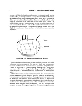
Continuum elements are the two- and three-dimensional solid elements.
Their formulation basis comes from the theory of elasticity. The theory of
elasticity provides the governing equations for the deformation and stress
response of a linear elastic continuum subjected to external loads. Few
closed form or numerical solutions exist for two-dimensional continuum
problems, and almost none exist for three-dimensional problems; this
makes the finite element method invaluable.
An extensive literature has developed since the 1960s when the term
"finite element" originated. The first textbook appeared in 1967 [see
Reference 1.1]. The number of books and conference proceedings published
since then is near two hundred and the number of journal papers and other
publications is in the thousands. The engineer beginning study of the finite
element method may consult references [1.2], [1.3], [1.4], [1.5], [1.6], [1.7],
or [1.8] for formulation [1.9], [1.10], [1.11], [1.12], [1.13], or [1.14] for
structural and solid mechanics applications, and [1.15], [1.16], or [1.17] for
computer algorithms and implementation.
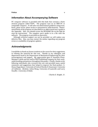
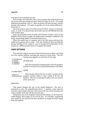
1.2 One-Dimensional Spring System
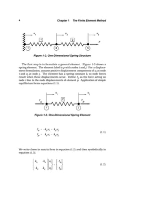
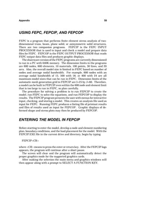
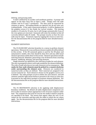
The fundamental operation of the finite element method is illustrated by
analysis of a one-dimensional spring system. A two-spring structure is
sketched in Figure 1-2. Each spring is an element identified by the number
in the box. The spring elements have a node at each end and they connect
at a common node. The number in the circle labels each node. The number
in the box labels each element. The subscripted u values are the node
displacements, i.e., degrees-of-freedom. There is an applied force F at node
3. We wish to solve for the node displacements and spring forces.](https://image.slidesharecdn.com/cekfeprimer-140910223214-phpapp01/85/Cek-fe-primer-10-320.jpg)
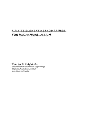
![Section 1.2 One-Dimensional Spring System 5
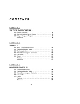
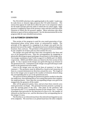
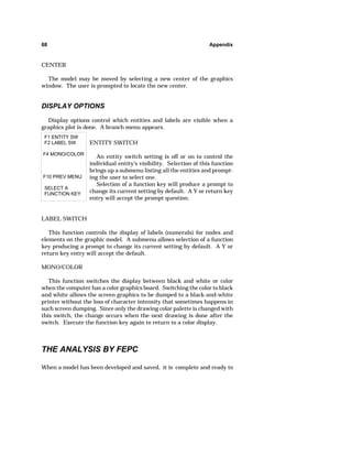
[k]{d} {f } (1.3)
Here, [k] is the element stiffness matrix, {d} is the element node displace-ment
vector, and {f} is the element node internal force vector. These steps
k1 k1
k1 k1
u1
u2
f11
f21
(1.4)
k2 k2
k2 k2
u2
u3
f22
f32
(1.5)
at node 1 ˆ forces 0 v f11 F1
at node 2 ˆ forces 0 v f21 f22 F2
at node 3 ˆ forces 0 v f32 F3
(1.6)
k1u1 k1u2 F1
k1u1 k1u2 k2u2 k2u3 F2
k2u2 k2u3 F3
(1.7)
complete the element formulation.
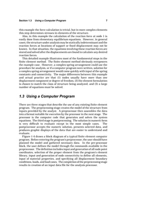
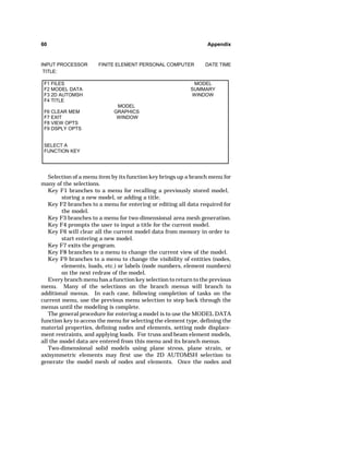
Now apply the general formulation to each element:
for element 1
and for element 2
The force components in the element equations are internal forces on the
nodes produced by the elements when the nodes displace. Equilibrium
requires that the sum of the internal forces equals the external force at
each node. Representing the external force by Fi, where i represents each
node, the equilibrium equations become:
Substitute the element equations for the internal force terms in the
equilibrium equations (1.6), and that, in effect, performs the structure
assembly and yields the structure equations (1.7).](https://image.slidesharecdn.com/cekfeprimer-140910223214-phpapp01/85/Cek-fe-primer-12-320.jpg)
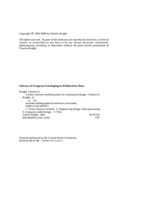
![6 Chapter 1 The Finite Element Method
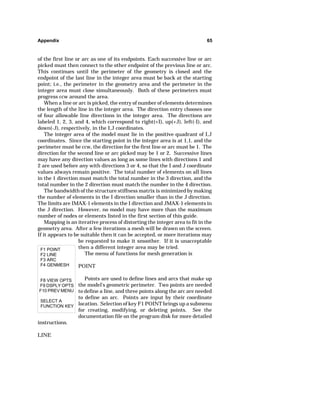
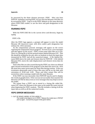
These are written in matrix form in equation (1.8) and symbolically in
equation (1.9) where [K] is the structure stiffness matrix, {D} is the
structure node displacement vector, and {F} is the structure external force
vector.
k1 k1 0
k1 k1k2 k2
0 k2 k2
u1
u2
u3
F1
F2
F3
(1.8)
[K]{D} {F} (1.9)
The set of structure or system equations must now be solved. The spring
constants of the springs are known, so all terms in the structure stiffness
matrix are known. The applied forces are known and the node displace-ments
become the unknowns in this set of three simultaneous equations.
We get the solution by premultiplying both sides of equation (1.9) by the
inverse of [K]. However, in this case the inverse of [K] is singular, meaning
that we cannot get a unique solution. Physically, this means that the
structure can be in equilibrium at any location in the x space, and it is free
to occupy any of those positions. This allows rigid body motion. To have a
unique solution we must locate the structure; that is, apply boundary
conditions such as a fixed displacement on one of the nodes which is enough
to prevent rigid body motion.
If an external force F applies to node 3, and the spring attaches to the
wall at node 1, then it is natural to set the displacement of node 1 to zero.
This action zeroes the first column of terms in the structure stiffness
matrix, and that leaves three equations with two unknowns. If the value
of the reaction force at node 1 is unknown, then we may skip the first
equation and choose the second and third equations to solve for the
unknown displacements. If the external force on node 2 is zero then
k1k2 k2
k2 k2
u2
u3
0
F
(1.10)
Now we may get the solution of the resulting equations (1.10) by
premultiplying both sides of the equation by the inverse of this reduced
structure stiffness matrix. Using the solved displacements, we calculate
each element internal force by use of the individual element equations. In](https://image.slidesharecdn.com/cekfeprimer-140910223214-phpapp01/85/Cek-fe-primer-13-320.jpg)
![8 Chapter 1 The Finite Element Method
PREPROCESSOR
INPUT DATA
Control Data, Materials, Node and Element
Definition, Boundary Conditions, Loads
FORM ELEMENT [k ]
Read Element Data, Calculate Element
Stiffness Matrix, [k ]
FORM SYSTEM [K ]
Assemble Element [k ]s to Form the
System Stiffness Matrix, [K ]
Element File
APPLY DISPLACEMENT BOUNDARY CONDITIONS
POSTPROCESSOR
Load File
Element File
COMPUTE DISPLACEMENTS
Solve the System Equations
[K ]{D } = {F }
for the Displacements
{D } = [K ] - 1{F }
COMPUTE STRESSES
Calculate Stresses and Output
Files for Postprocessor Plotting
Load File
Displacement,
Stress Files
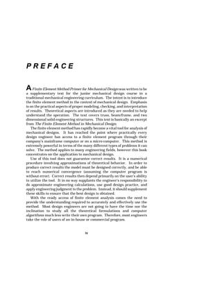
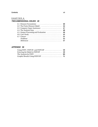
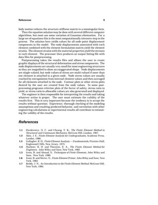
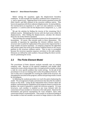
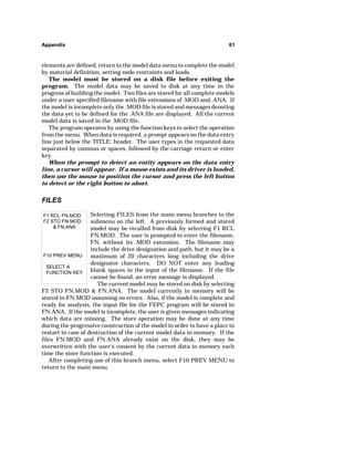
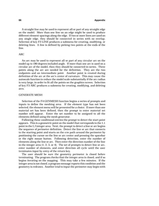
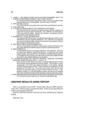
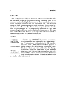
Figure 1-4. Finite Element Computer Program Block Diagram
The processor reads from the input data file each element definition,
calculates terms of the element stiffness matrix, and stores them in a data
array or on a disk file. The element type selection determines the form of
the element stiffness matrix. The next step is to assemble the structure
stiffness matrix by matrix addition of all element stiffness matrices. The
application of enough displacement boundary conditions to prevent rigid](https://image.slidesharecdn.com/cekfeprimer-140910223214-phpapp01/85/Cek-fe-primer-15-320.jpg)
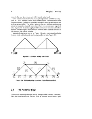
![12 Chapter 2 Trusses
A one-dimensional truss element then has an element formulation
identical to the one-dimensional spring given in equation (1.2). This is its
element stiffness matrix for one-dimensional displacement and loading
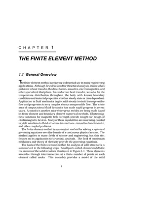
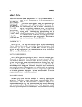
along the axis of the member. For member positioning in a two-dimen-sional
space as illustrated in Figure 2-1, each node has two components of
displacement u and v and two components of force p and q. This leads to
a set of element equations with an element stiffness matrix of size 4 by 4.
Figure 2-1. Two-Dimensional Truss Element
Derivation of the two-dimensional element stiffness matrix comes
through coordinate transformations [2.1], but first we expand the one-dimensional
stiffness matrix to two dimensions with the member lying
along the x axis. Assuming an order of components and equations of u and
v at node i followed by u and v at node j, the element equations are written
in equation (2.2).
k 0 k 0
0 0 0 0
k 0 k 0
0 0 0 0
ui
vi
uj
vj
pi
qi
pj
qj
(2.2)
Notice that the terms relating displacement and force in the x direction](https://image.slidesharecdn.com/cekfeprimer-140910223214-phpapp01/85/Cek-fe-primer-19-320.jpg)
![Section 2.1 Direct Element Formulation 13
are the spring constant of the member and the terms relating displacement
and force in the y direction are zero. A linear analysis always assumes that
the displacements are much smaller than the overall geometry of the
structure; therefore, the stiffness is based on the undeformed configuration.
In this case, because it is a motion perpendicular to the line of the member,
if we consider a vertical displacement component at one of the nodes, no
vertical force results because there is no axial stretch relative to the
undeformed configuration.
This formulation represents the element stiffness matrix in a local
element coordinate system that is aligned with the element axis. To
position the element at an arbitrary angle, O, from the x coordinate axis, we
perform a transformation of coordinate systems to derive the element
stiffness matrix in the x,y global coordinate system. In the system of
equations, the displacements and forces are both vectors, so they transform
through standard vector transformations. The displacement components
in global coordinates relate to local components through equation (2.3).
{d} [T]{dk } (2.3)
Here, {d'} are the global displacement components, [T] is the transforma-tion
matrix, and {d} are the local element coordinate displacement
[T]
c s 0 0
s c 0 0
0 0 c s
0 0 s c
(2.4)
{f } [T]{f k} . (2.5)
[k]{d} {f } . (2.6)
components.
The transformation matrix is given by equation (2.4).
Here, s is the sin O, and c is the cos O. Similarly, the force components in
the global coordinate system are given by
The element stiffness matrix in the local coordinate system is defined in
matrix notation from equation (2.2) by](https://image.slidesharecdn.com/cekfeprimer-140910223214-phpapp01/85/Cek-fe-primer-20-320.jpg)
![14 Chapter 2 Trusses
Making the substitutions for {d} and {f} given above yields
[k][T]{dk } [T]{f k} . (2.7)
The transformation matrix is an orthogonal matrix, meaning that
[T]1
[T]— . (2.8)
Therefore, multiplying equation (2.7) by [T]— produces
[T]— [k][T]{dk} {f k } (2.9)
which makes
[kk ] [T]—[k][T] k
c 2 cs c 2 cs
cs s 2
cs s 2
c 2 cs c 2 cs
cs s 2 cs s 2
(2.10)
The use of this element formulation and equation assembly is shown
through the example truss structure pictured in (2.11). The elements and
nodes are numbered, and load and boundary conditions are shown. The
structure equations are
[K]{D} {F} (2.11)
where, [K] is the structure stiffness matrix, {D} is the node displacement
vector, and {F} is the applied load vector.
These equations come from applying the conditions of equilibrium to all
the nodes by setting the summation of internal forces equal to the applied
forces. The internal forces are given by the product of each element
stiffness matrix with its node displacements. This yields equation (2.12),
where the subscripts refer to the numbered elements. If the displacement
vector in each term of the equation above was identical, then we could
[k]{d}|1 [k]{d}|2 [k]{d}|3 {F} (2.12)](https://image.slidesharecdn.com/cekfeprimer-140910223214-phpapp01/85/Cek-fe-primer-21-320.jpg)
![Section 2.1 Direct Element Formulation 15
Figure 2-2. Example Truss Structure
factor it out and add the stiffness matrices term-by-term to produce the
structure stiffness matrix.
all the structure degrees-of-freedom, not just the ones associated with a
given element. In order for the matrix equation to be correct, a corre-sponding
expansion of the displacement vector. It expands to the size of the
structure stiffness matrix which in this example becomes a 6-by-6 matrix.
The expansion simply adds rows and columns of zeroes to each element
stiffness matrix corresponding to the additional structure degrees-of-freedom
The displacement vector for each element must then expand to include
expansion of the element stiffness matrix must accompany the
0 0 0 0
0 k1 0 k1
0 0 0 0
0 k1 0 k1
0 0 0 0 0
0 0 0 0 0
0 0 0 0 0
0 0 0 k1 0
0 0 0 0 0
0 0 0 k1 0
(2.13)
unused in the given element [2.1].
Applying this approach, the stiffness matrix for element 1 in the example
results from using equation (2.10) with a O value of 90 degrees. Rows and
columns of zeroes fill in equations and positions involving u1 and v1 as
shown in equation (2.13).
Similarly, the matrix for element 2 with O equal to 135 degrees and rows](https://image.slidesharecdn.com/cekfeprimer-140910223214-phpapp01/85/Cek-fe-primer-22-320.jpg)
![16 Chapter 2 Trusses
and columns filled in equations and positions involving u2 and v2 results in
equation (2.14).
[k]2
.5k2 .5k2 0 0 .5k2 .5k2
.5k2 .5k2 0 0 .5k2 .5k2
0 0 0 0 0 0
0 0 0 0 0 0
.5k2 .5k2 0 0 .5k2 .5k2
.5k2 .5k2 0 0 .5k2 .5k2
(2.14)
Finally for element 3, O is 0 degrees and u3 and v3 are the additional
[k]3
k3 0 k3 0 0 0
0 0 0 0 0 0
k3 0 k3 0 0 0
0 0 0 0 0 0
0 0 0 0 0 0
0 0 0 0 0 0
(2.15)
[K]
.5k2k3 .5k2 k3 0 .5k2 .5
.5k2 .5k2 0 0 .5k2 .
k3 0 k3 0 0
0 0 0 k1 0
.5k2 .5k2 0 0 .5k2 .
.5k2 .5k2 0 k1 .5k2 .5k
(2.16)
degrees-of-freedom in equation (2.15).
The summations of equation (2.12) are now carried out by adding the
expanded element stiffness matrices term-by-term. The resulting structure
stiffness matrix is in equation (2.16).](https://image.slidesharecdn.com/cekfeprimer-140910223214-phpapp01/85/Cek-fe-primer-23-320.jpg)
![Section 2.3 The Analysis Step 19
results. Some of them are inherent in the computer hardware and
software, but some of them are under user control. For small truss
structure models, most programs have enough numerical accuracy and
performance to provide an accurate solution without much user concern.
Large models cause the most concern [2.1].
A large model is one in which there are many elements and nodes used
to represent the structure. (The structure itself is not necessarily large.)
With many system equations it becomes difficult to find a numerical
solution if the equation matrix is full. Even the inverse of a 10-by-10
matrix may be inaccurate if done by Gauss elimination with only a few
significant figures carried along in the mathematical operations. The
accuracy will improve, however, if the matrix has its nonzero terms
clustered near the diagonal. This reduces the number of operations and
reduces the roundoff error carried along in each operation. This kind of
matrix, with its nonzero terms near the diagonal, is a banded matrix.
If the truss structure model consists of thousands of nodes and elements,
then the bandwidth of the structure equations needs to be small. Keeping
it small reduces error and computing time. If the mesh plan does not have
a small bandwidth for the system of equations, then bandwidth minimizers
available in many programs should reduce it. There are several algorithms
available which will usually, but not always, find a better node or element
numbering pattern. Most programs keep the original numbering in the
model for documentation and presentation purposes by storing the
renumbered nodes and elements in translation tables. In some programs
the user has the option to keep the original numbering or change to the
new numbering plan.
The approximation error for the truss element is zero since the element
formulation is in exact agreement with the assumptions used to define a
truss member. During processor execution there are usually some prompts
of progress made displayed on the computer, and if errors occur, messages
appear. Sometimes these messages have meaning only to the computer
program developer, but some of them can be very helpful in determining
the model error.
The most common runtime errors involve incorrect definition of elements
or incorrect application of displacement boundary conditions. For example,
both conditions can produce an error message that the structure stiffness
matrix is not positive-definite or that a negative pivot or diagonal term in
the stiffness matrix appeared during equation reduction. For truss models
this can occur whenever there are not enough boundary conditions to
prevent rigid body motion. It can also occur when two elements connect in-line
resulting in zero lateral stiffness. It can also mean that the truss
structure itself is not kinematically stable associated with a kinematic
linkage of the members.
The error messages from the computer program should provide an
associated element number, node number, or equation number where the](https://image.slidesharecdn.com/cekfeprimer-140910223214-phpapp01/85/Cek-fe-primer-26-320.jpg)
![Section 2.5 Case Study 21
additional model refinements and whether the results have converged to
enough accuracy. For truss structures we know that the element formula-tion
is exact; therefore, in a correctly defined and processed model the
output results will be exact. So there is no need for refined modeling to
produce converged results in this case, but the modeling of loads and
boundary conditions may not be fully appropriate.
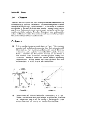
It is important to remember that this is a linear elastic analysis. One of
the potential failure modes is overstressing while another is elastic
buckling. The stresses compare to yield strength for the material to
determine if overstress failure occurs. To determine whether there is
potential for elastic buckling, the user must identify the members with a
significant compression load, and then use Euler buckling equations from
mechanics of materials to evaluate the potential for each member to buckle
[2.2]. This is not done in a linear elastic analysis computer program. If any
member has an inadequate safety factor against buckling, then the entire
structure should have a stability analysis conducted using a solution
algorithm available in some nonlinear computer codes.
2.5 Case Study
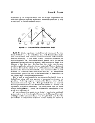
We show a typical truss structure in Figure 2-5. This structure has
members of two different cross-section areas and two different materials.
The mesh plan for this structure is illustrated in Figure 2-6 with a chosen
pattern for node and element numbers. The enforced boundary conditions
Figure 2-5. Two-Dimensional Truss Structure](https://image.slidesharecdn.com/cekfeprimer-140910223214-phpapp01/85/Cek-fe-primer-28-320.jpg)

![C H A P T E R 3
BEAMS AND FRAMES
Application of straight beam theory readily solves simple beam problems
especially if the problem is statically determinant. If the beam is not
particularly simple, in that it may have cross-section changes, multiple
supports, or complex loading distributions, then we can use beam theory,
but it is very tedious to develop the solution by hand. Also, many 2-D or 3-
D framework structures may require solutions in which the truss member
assumption is inadequate and therefore needs the beam flexure formula-tion.
Further applications may include beam members as re-inforcement
members in combination beam, plate, and shell structures. These
applications are readily attacked with the finite element formulation.
3.1 Element Formulation
Here we follow the direct approach for formulating the element stiffness
matrix [3.1]. The element equations relating general displacement and
force components are given by
[k]{d} {f } (3.1)
where [k] is the element stiffness matrix, {d} is the node displacement
component column matrix, and {f} is the internal force component column
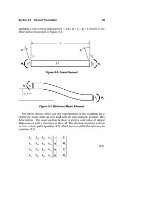
matrix. The stiffness matrix terms derive from superposition of simple
beam solutions. Apply a unit displacement of one component with the other
components held to zero and evaluate the magnitude of resulting force
components. For example, taking the element shown in Figure 3-1 and
28](https://image.slidesharecdn.com/cekfeprimer-140910223214-phpapp01/85/Cek-fe-primer-35-320.jpg)
![30 Chapter 3 Beams and Frames
k11 Fi , k21 Mi , k31 Fj , and k41 M (3.3)
Using superposition of beam deflection equations available in any
mechanics of materials text, we write equations (3.4). Solve these
equations for the values of Fi and Mi in equations (3.5).
vi 1
FiL3
3EI
MiL2
2EI
ki 0
FiL2
2EI
MiL
EI
(3.4)
Fi
12EI
L3
Mi
6EI
L2
(3.5)
Use static equilibrium equations to get the values of Fj and Mj in equation
(3.6).
Fj
12EI
L3
Mj
6EI
L2 (3.6)
We now have all the terms of column 1 of the 4x4 element stiffness
[k]
12EI
L3
... ... ...
6EI
L2
... ... ...
12EI
L3
... ... ...
6EI
L2
... ... ...
(3.7)
matrix as shown in equation (3.7).](https://image.slidesharecdn.com/cekfeprimer-140910223214-phpapp01/85/Cek-fe-primer-37-320.jpg)
![Section 3.1 Element Formulation 31
Similarly applying a unit value of rotation for ki and fixing all other
components to zero, we derive the force and moment values in Figure 3-3.
These come from superposition of the same solutions for end load and
moment to satisfy the displacement conditions.
Figure 3-3. Deformed Beam Element
Notice that the sign convention employed here is common in the finite
element formulation such that the component's sign always agrees with the
positive direction of a right-handed coordinate system. This does not agree
with most beam sign conventions employed in mechanics of material texts.
Therefore, the user should be aware that the output components will
normally be expressed using this finite element sign convention. This
means, for example, that a positive value of moment at the first node of the
element will produce a tensile stress at the top surface of the beam. In
contrast, a positive moment on the second node will produce a compressive
stress at the top surface of the beam.
Obtain the remaining terms in the stiffness matrix by application of the
same procedures to the second node. The final element stiffness is then
given in equation (3.8).
[k]
12EI
L3
6EI
L2
12EI
L3
6EI
L2
6EI
L2
4EI
L
6EI
L2
2EI
L
12EI
L3
6EI
L2
12EI
L3
6EI
L2
6EI
L2
2EI
L
6EI
L2
4EI
L
(3.8)](https://image.slidesharecdn.com/cekfeprimer-140910223214-phpapp01/85/Cek-fe-primer-38-320.jpg)
![32 Chapter 3 Beams and Frames
This formulation provides an exact representation of a beam span within
the assumptions involved in straight beam theory, provided there are no
loads applied along the span. Therefore, in modeling considerations, place
a node at all locations where concentrated forces, or moments, act in
creating the element assembly. In spans where there is a distributed load,
the assumed displacement field does not completely satisfy the governing
differential equation; therefore, the solution is not exact but approximate.
One approach to modeling in this area is to make enough subdivisions of
the span with distributed load to lessen the error. If a work equivalent load
set acting on the nodes replaces the distributed load, then the influence of
any error in this element will not propagate to other elements. In other
words, the displacement components at the nodes will be correct if we use
the equivalent load set. The equivalent load components for a distributed
load on the element span are the negative of the end reaction force and
moment found in the solution of a fixed end beam with the same distrib-uted
load as shown by Logan [3.2].
This formulation provides the ability to analyze simple beams, but does
not account for the axial load that may exist in beam members connected
in a framework. By adding the truss element formulation by superposition
with the previous formulation, we have an element that can support both
lateral and axial loads. The axial stiffness terms at each node are added
to the element stiffness matrix formulation to create the frame element
stiffness matrix in equation (3.9).
[k]
AE
L
0 0
AE
L
0
0 12EI
L3
6EI
L2
0
12EI
L3
0 6EI
L2
4EI
L
0
6EI
L2
AE
L
0 0 AE
L
0
0
12EI
L3
6EI
L2
0 12EI
L3
0 6EI
L2
2EI
L
0
6EI
L2
(3.9)
This assumes that superposition is valid for this case. If displacements
are small it will be accurate; however, there is an interaction that occurs](https://image.slidesharecdn.com/cekfeprimer-140910223214-phpapp01/85/Cek-fe-primer-39-320.jpg)
![Section 3.2 The Finite Element Model 33
between axial and lateral loading on beams. If the axial load is tensile it
reduces the effect of lateral loads, and when the axial load is compressive
it amplifies the effect of lateral loads. To gain further information on this
interaction, consult an advanced mechanics of materials text [3.3] for the
equations that apply to members called beam-columns or struts. The
equations for these members are a nonlinear function of the size of lateral
displacement. Therefore, a linear analysis cannot account for the effect.
The user should be aware of this consideration. Remember that if the
axial load is tensile, the results from beam elements will be higher than
they actually are; thus results are conservative. Also, if the axial load is
compressive, the results will be less than actual and may be in serious
error. The size of error associated with the compressive loading is normally
quite small until the axial load exceeds roughly 25 percent of the Euler
column buckling load. In most cases a design should have a factor of safety
against buckling greater than four anyway.
Now the formulation includes the u and v displacement components and
the section rotation at the nodes in the element local coordinate system.
Using the coordinate transformations developed for truss members, we may
orient this two-dimensional beam element in 2-D space. Through this
transformation, then, the element formulation applies to any 2-D frame-work.
3.2 The Finite Element Model
In planning the mesh for a structure to be modeled with beam elements,
the factors just revealed in element formulation provide guidance about the
proper element subdivision and connections. Since the element formulation
is exact for a beam span with no intermediate loads, then we need only one
element to model any member of the structure that has constant cross-section
properties and no intermediate loads. Where a span has a
distributed load, we may subdivide it with several elements to lessen the
error depending on the solution accuracy desired.
There should be a node placed at every location in the structure where
a point load is applied. Also, where frame members connect such that the
line element changes direction or cross-section properties change, we should
place a node and end an element at that point. Remember that the
connection of two or more elements at a node guarantees that each element
connecting at that node will have the same value of linear and rotation
displacement components at that node. Physically, think of this as a solid,
continuous, or welded configuration.](https://image.slidesharecdn.com/cekfeprimer-140910223214-phpapp01/85/Cek-fe-primer-40-320.jpg)
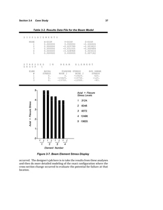
![34 Chapter 3 Beams and Frames
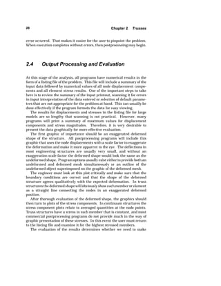
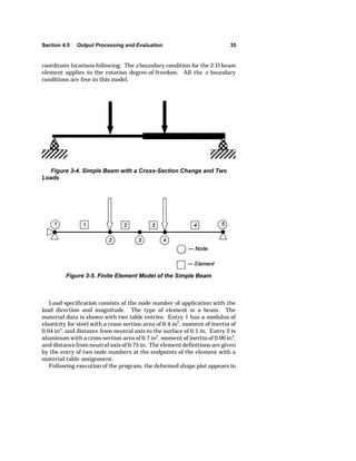
3.3 Output Processing and Evaluation
A complete printout, or listing file, lists a reflection of model input data, the
displacement results including rotations, and output of stresses resulting
from moment, axial, and shear forces. The graphical presentation of the
deformed shape ideally would use the rotations at the nodes with the
assumed displacement shape function for the element to plot the actual
curved shape the elements take when loaded. However, most programs
only plot the deformed shape using the node translation displacements and
straight line connections to represent the elements. In this case it is
difficult to determine from the graphic if we applied the rotational
boundary conditions. In order to check boundary conditions and get a
smooth visualization of the deformation curvatures, the user may resort to
remodeling with several element subdivisions within each span.
The stresses in 2-D beam elements consist of a normal stress acting
normal to the beam cross section and a transverse shear stress acting on
the face of the cross section. The normal stress comes from superposition
of the axial stress that is uniform across the section with the bending stress
due to the moment on the section. This combination will result in the
maximum normal stress occurring either at the top or bottom surface. The
transverse shear stress is usually an average across the cross section
calculated by the transverse load divided by the area. This obviously does
not account for the shear stress variation that occurs across the section
from top to bottom [3.3]. The transverse shear stress must be zero at the
top and bottom surfaces and has some nonuniform distribution in between
that is a function of the cross-section geometry. This variation is usually
of minor importance, but the analyst may calculate it if desired.
Most of the available finite programs do not make graphical presentation
of the beam stress results. So it reverts to the engineer to evaluate the
stress output usually based on values from the printout listing. The
engineer also must check for Euler buckling in members that have an axial
compressive stress. If the factor of safety against buckling in these mem-bers
is less than about 4, then the stresses may need correction for the
interaction between the axial and flexural stress in that member.
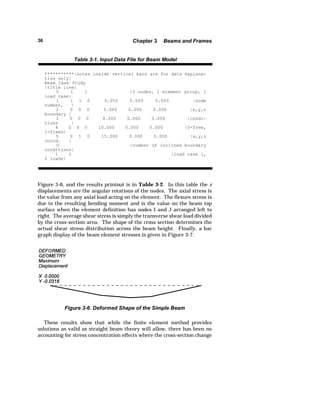
3.4 Case Study
We show a simple beam structure in Figure 3-4 with two different cross
sections and two loads. It has simple supports, and we develop a mesh plan
in Figure 3-5 with five nodes and four elements. The model input data list
is in Table 3-1. The title line is first with the control data line next. Node
definition begins with its number, then boundary condition restraints and](https://image.slidesharecdn.com/cekfeprimer-140910223214-phpapp01/85/Cek-fe-primer-41-320.jpg)
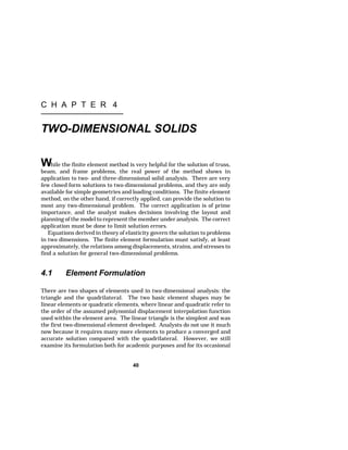
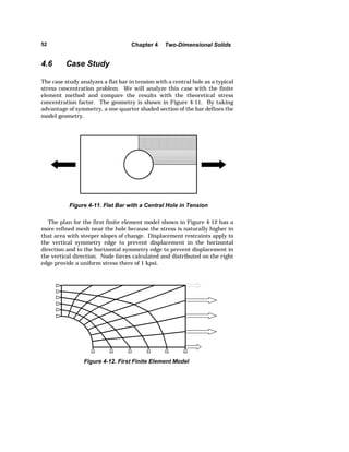
![42 Chapter 4 Two-Dimensional Solids
This displacement formulation also satisfies the compatibility require-ments
in the theory of elasticity [4.1] for the continuum. The compatibility
requirements are that no gaps or overlaps of material may occur during the
process of deformation under load. From these equations, we can see that
the continuous nature of the function enforces compatibility within the
element. On a triangular element, since the interpolation is linear, any
edge formed by connecting two nodes that is a straight line before
deformation will remain a straight line after deformation. Therefore, any
connecting element using the same two nodes for its shared edge satisfies
compatibility.
Some of the early finite element programs [4.2] used the triangle
element to create a quadrilateral element by subdividing a quadrilateral
shape into four triangles using the centroid of the quadrilateral as their
apex. After finding the stiffness matrix for each triangle element, assembly
of the triangles and condensation of the internal node resulted in the
stiffness matrix of the quadrilateral element. This was an effective way to
use the triangular element formulation and employ many more elements
without tedious input. However, the element of choice now is an
isoparametric quadrilateral formulation.
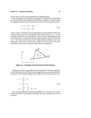
Next we examine the displacement basis for formulation of the isopara-metric
quadrilateral element. Taig [4.3] developed the element, and Irons
[4.4] published its formulation. The quadrilateral element formulation
derives from the formulation of a square element. It uses a co-ordinate
system transformation to convert the square to a quadrilateral. Begin with
the square element shown in Figure 4-2 with corner nodes.
Figure 4-2. Square Two-Dimensional Finite Element
Recognizing that four constants can be evaluated with four nodes, a
logical expression for the displacement function components becomes](https://image.slidesharecdn.com/cekfeprimer-140910223214-phpapp01/85/Cek-fe-primer-49-320.jpg)
![Section 4.2 The Finite Element Model 45
This is the first step in the p-convergence method for numerical convergence
on the correct solution. The user may easily use h-convergence by successive
model building in all finite element programs. However, there are usually
only linear and quadratic order elements in the element library of most
programs that limit the pursuit of p-convergence. There are several new
commercial codes becoming available now, and a recent text by Szabo and
Babuska [4.5] provides good coverage of the p-convergence method theory
and application.
In planning the mesh, try to use symmetry whenever possible. The
advantages include a reduction of labor of model input, reduction of
computer time and cost, and a decrease in computer round-off error in the
equation solution because fewer equations exist in the model. There are
some drawbacks. Sometimes it becomes more difficult to picture the model.
Also, peak stresses may occur along symmetry lines and make it difficult to
locate elements properly to show the peak.
Recognize symmetry in two-dimensional objects by observation of
geometric patterns that may occur. These may develop by incrementing
plane sections, rotating sections about an axis, periodically rotating sections
about an axis, or by reflecting a section about a plane. For the symmetric
model to provide a solution, the load distribution must also be symmetric on
the object. In some cases, we can find solutions for anti-symmetric loading
conditions on symmetric objects by proper imposition of displacement
boundary conditions.
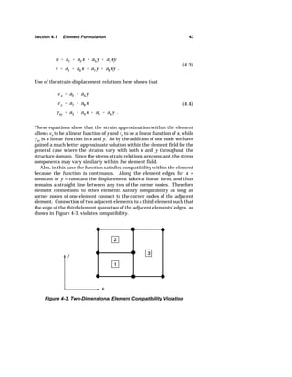
Displacement boundary conditions enforce symmetry by restricting node
points that lie on lines of symmetry to motion along the line of symmetry.
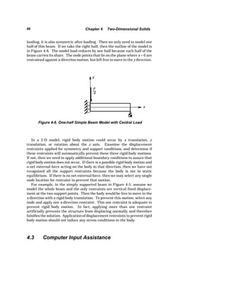
For example, look at the simply supported beam with central load in Figure
4-5. It has a vertical plane of symmetry at coordinate x = 0.
Figure 4-5. Simple Beam with Central Load
When the load applies, the beam will deflect downward and the displace-ment
of every material particle in the right half will be a mirror image of the
corresponding particle in the left half. So if the body is symmetric before](https://image.slidesharecdn.com/cekfeprimer-140910223214-phpapp01/85/Cek-fe-primer-52-320.jpg)
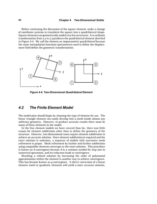
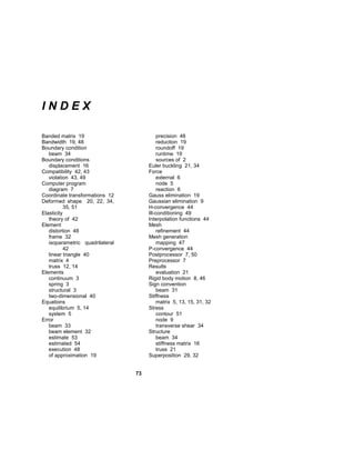
![Section 4.4 The Analysis Step 49
Figure 4-8. (Continued)
element compatibility violations, and stiffness matrix ill-conditioning caused
by large differences in stiffness values of elements [4.6]. Examples of severe
element distortion of quadrilateral elements are shown in Figure 4-9.
Ideally the elements would remain close to square shape. High aspect
ratios, large differences in side length, and very small or large inside angles
all contribute to numerical precision errors. In fact, inside angles greater
than 180 degrees may cause negative stiffnesses. Most commercial
programs will check the element distortion and issue warning messages or
cancel execution if the distortion is too high.
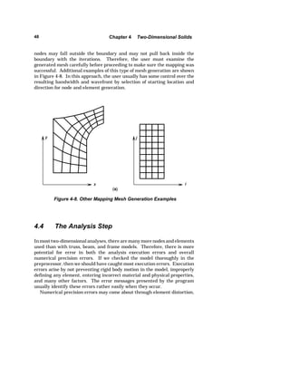
Even though most two-dimensional element formulations guarantee
satisfaction of the compatibility requirements in theory of elasticity,
modeling errors may still violate compatibility. Some of these are illustrated
in Figure 4-10.
To satisfy compatibility in corner-noded elements, each element side may
only join to a side of one other element. For elements with midside nodes,
each must connect to another element at the corners, and all three nodes on
a side must connect by use of common nodes.
The solution accuracy in two-dimensional analyses is very dependent on
the user's ability to evaluate the results and produce a numerically
converged solution. In the truss and beam elements, the element formula-tion
was exact, and therefore there was no concern about interpolation
accuracy. However, these two-dimensional elements require numerical](https://image.slidesharecdn.com/cekfeprimer-140910223214-phpapp01/85/Cek-fe-primer-56-320.jpg)


The document is a primer on the finite element method for mechanical design, intended as a supplementary text for mechanical engineering courses. It focuses on practical modeling, evaluation, and interpretation of results while introducing theoretical concepts as needed. The text emphasizes the importance of correct modeling and user skill to ensure accurate results, highlighting the method's applications in trusses, beams, frames, and solid structures.