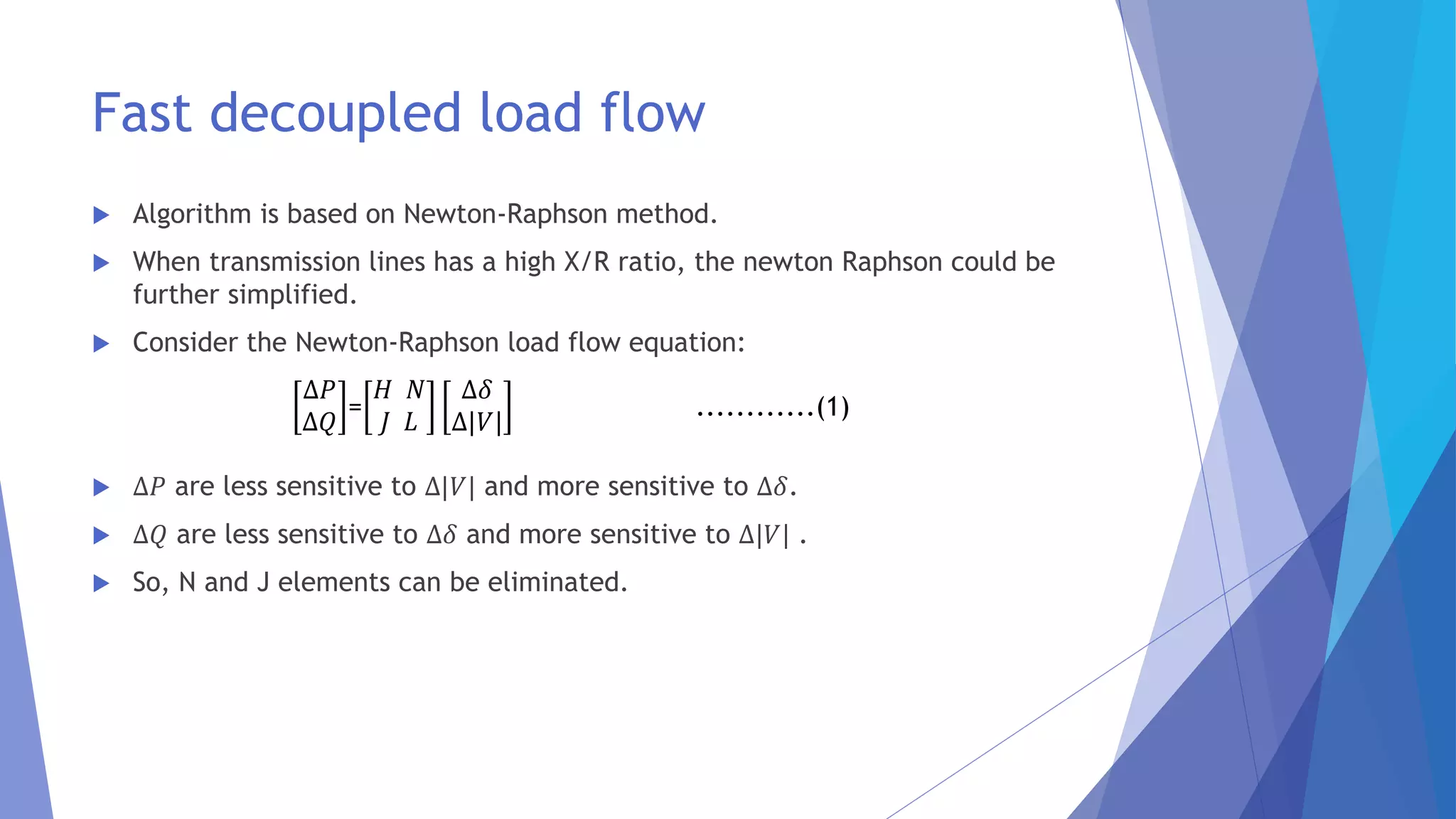
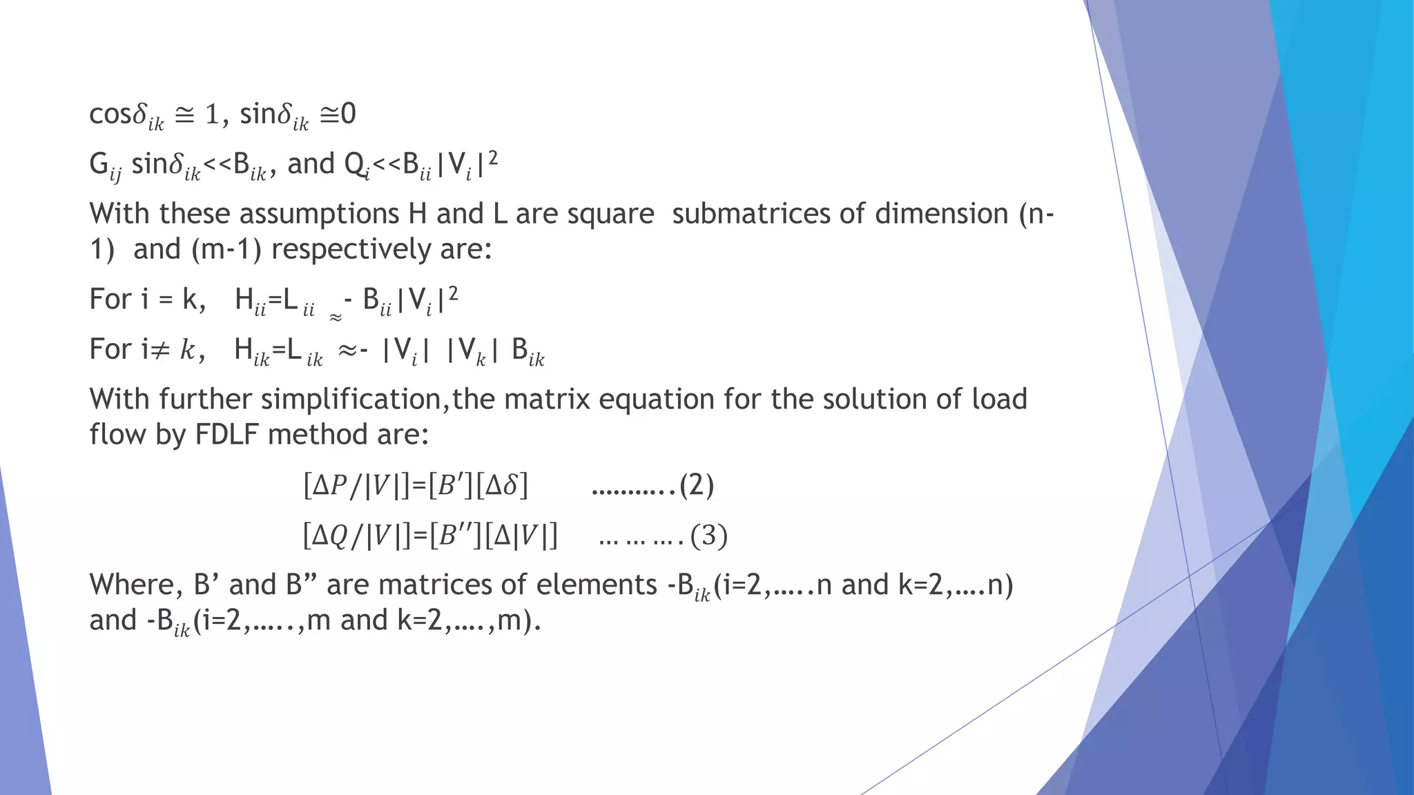
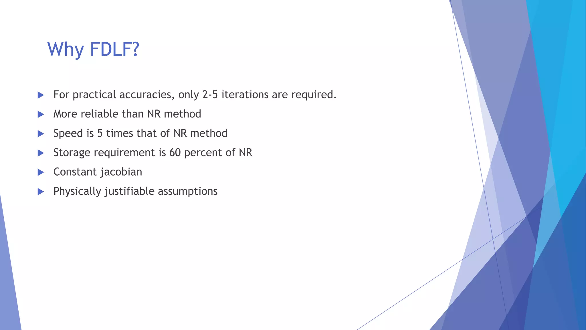
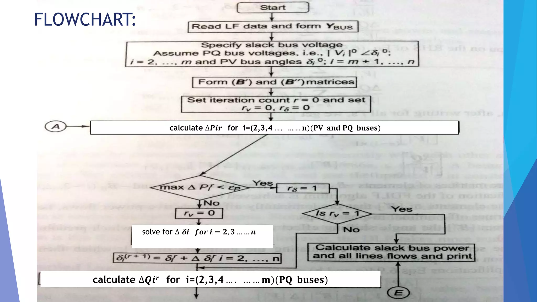
Load Flow Study
Fast Decoupled Load Flow(FDLF)
Presented by-
fs
Overview
 Fast decoupled load flow
 Why FDLF?
 Flowchart
 Program
 Output
 Conclusion
 Reference
Fast decoupled load flow
 Algorithm is based on Newton-Raphson method.
 When transmission lines has a high X/R ratio, the newton Raphson could be
further simplified.
 Consider the Newton-Raphson load flow equation:
 ∆𝑃 are less sensitive to ∆|𝑉| and more sensitive to ∆𝛿.
 ∆𝑄 are less sensitive to ∆𝛿 and more sensitive to ∆|𝑉| .
 So, N and J elements can be eliminated.
∆𝑃
∆𝑄
=
𝐻 𝑁
𝐽 𝐿
∆𝛿
∆|𝑉|
............(1)
cos𝛿𝑖𝑘 ≅ 1, sin𝛿𝑖𝑘 ≅0
G𝑖𝑗 sin𝛿𝑖𝑘<<B𝑖𝑘, and Q𝑖<<B𝑖𝑖|V𝑖|2
With these assumptions H and L are square submatrices of dimension (n-
1) and (m-1) respectively are:
For i = k, H𝑖𝑖=L 𝑖𝑖 ≈
- B𝑖𝑖|V𝑖|2
For i≠ 𝑘, H𝑖𝑘=L 𝑖𝑘 ≈- |V𝑖| |V 𝑘| B𝑖𝑘
With further simplification,the matrix equation for the solution of load
flow by FDLF method are:
∆𝑃/|𝑉| = 𝐵′ ∆𝛿 ………..(2)
∆𝑄/|𝑉| = 𝐵′′ ∆|𝑉| … … … . (3)
Where, B’ and B” are matrices of elements -B𝑖𝑘(i=2,…..n and k=2,….n)
and -B𝑖𝑘(i=2,…..,m and k=2,….,m).
Why FDLF?
 For practical accuracies, only 2-5 iterations are required.
 More reliable than NR method
 Speed is 5 times that of NR method
 Storage requirement is 60 percent of NR
 Constant jacobian
 Physically justifiable assumptions
FLOWCHART:
calculate ∆𝑷𝒊𝒓 for i=(2,3,4 … . … … 𝐧)(𝐏𝐕 𝐚𝐧𝐝 𝐏𝐐 𝐛𝐮𝐬𝐞𝐬)
solve for ∆ 𝜹𝒊 𝒇𝒐𝒓 𝒊 = 𝟐, 𝟑 … … 𝒏
calculate ∆𝑸𝒊 𝒓 for i=(2,3,4 … . … … 𝐦)(𝐏𝐐 𝐛𝐮𝐬𝐞𝐬)
Solve for ∆|Vi| for i=2,3 … . … . m.
PROGRAM-
fdlf.txt
OUTPUT-
Conclusion
 Due to constant jacobian, defining functions are not sensitive to any humps.
 It can be employed in optimization studies.
 Used for obtaining information of both real and reactive power for multiple
load flow studies.
References
 M. A.PAI , Computer Techniques in Power System Analysis.
 D.P. Kothari, Modern Power System Analysis .
THANK YOU!!!

Load flow study

  • 1.
    Load Flow Study FastDecoupled Load Flow(FDLF) Presented by- fs
  • 2.
    Overview  Fast decoupledload flow  Why FDLF?  Flowchart  Program  Output  Conclusion  Reference
  • 3.
    Fast decoupled loadflow  Algorithm is based on Newton-Raphson method.  When transmission lines has a high X/R ratio, the newton Raphson could be further simplified.  Consider the Newton-Raphson load flow equation:  ∆𝑃 are less sensitive to ∆|𝑉| and more sensitive to ∆𝛿.  ∆𝑄 are less sensitive to ∆𝛿 and more sensitive to ∆|𝑉| .  So, N and J elements can be eliminated. ∆𝑃 ∆𝑄 = 𝐻 𝑁 𝐽 𝐿 ∆𝛿 ∆|𝑉| ............(1)
  • 4.
    cos𝛿𝑖𝑘 ≅ 1,sin𝛿𝑖𝑘 ≅0 G𝑖𝑗 sin𝛿𝑖𝑘<<B𝑖𝑘, and Q𝑖<<B𝑖𝑖|V𝑖|2 With these assumptions H and L are square submatrices of dimension (n- 1) and (m-1) respectively are: For i = k, H𝑖𝑖=L 𝑖𝑖 ≈ - B𝑖𝑖|V𝑖|2 For i≠ 𝑘, H𝑖𝑘=L 𝑖𝑘 ≈- |V𝑖| |V 𝑘| B𝑖𝑘 With further simplification,the matrix equation for the solution of load flow by FDLF method are: ∆𝑃/|𝑉| = 𝐵′ ∆𝛿 ………..(2) ∆𝑄/|𝑉| = 𝐵′′ ∆|𝑉| … … … . (3) Where, B’ and B” are matrices of elements -B𝑖𝑘(i=2,…..n and k=2,….n) and -B𝑖𝑘(i=2,…..,m and k=2,….,m).
  • 5.
    Why FDLF?  Forpractical accuracies, only 2-5 iterations are required.  More reliable than NR method  Speed is 5 times that of NR method  Storage requirement is 60 percent of NR  Constant jacobian  Physically justifiable assumptions
  • 6.
    FLOWCHART: calculate ∆𝑷𝒊𝒓 fori=(2,3,4 … . … … 𝐧)(𝐏𝐕 𝐚𝐧𝐝 𝐏𝐐 𝐛𝐮𝐬𝐞𝐬) solve for ∆ 𝜹𝒊 𝒇𝒐𝒓 𝒊 = 𝟐, 𝟑 … … 𝒏 calculate ∆𝑸𝒊 𝒓 for i=(2,3,4 … . … … 𝐦)(𝐏𝐐 𝐛𝐮𝐬𝐞𝐬)
  • 7.
    Solve for ∆|Vi|for i=2,3 … . … . m.
  • 8.
  • 9.
    Conclusion  Due toconstant jacobian, defining functions are not sensitive to any humps.  It can be employed in optimization studies.  Used for obtaining information of both real and reactive power for multiple load flow studies.
  • 10.
    References  M. A.PAI, Computer Techniques in Power System Analysis.  D.P. Kothari, Modern Power System Analysis .
  • 11.