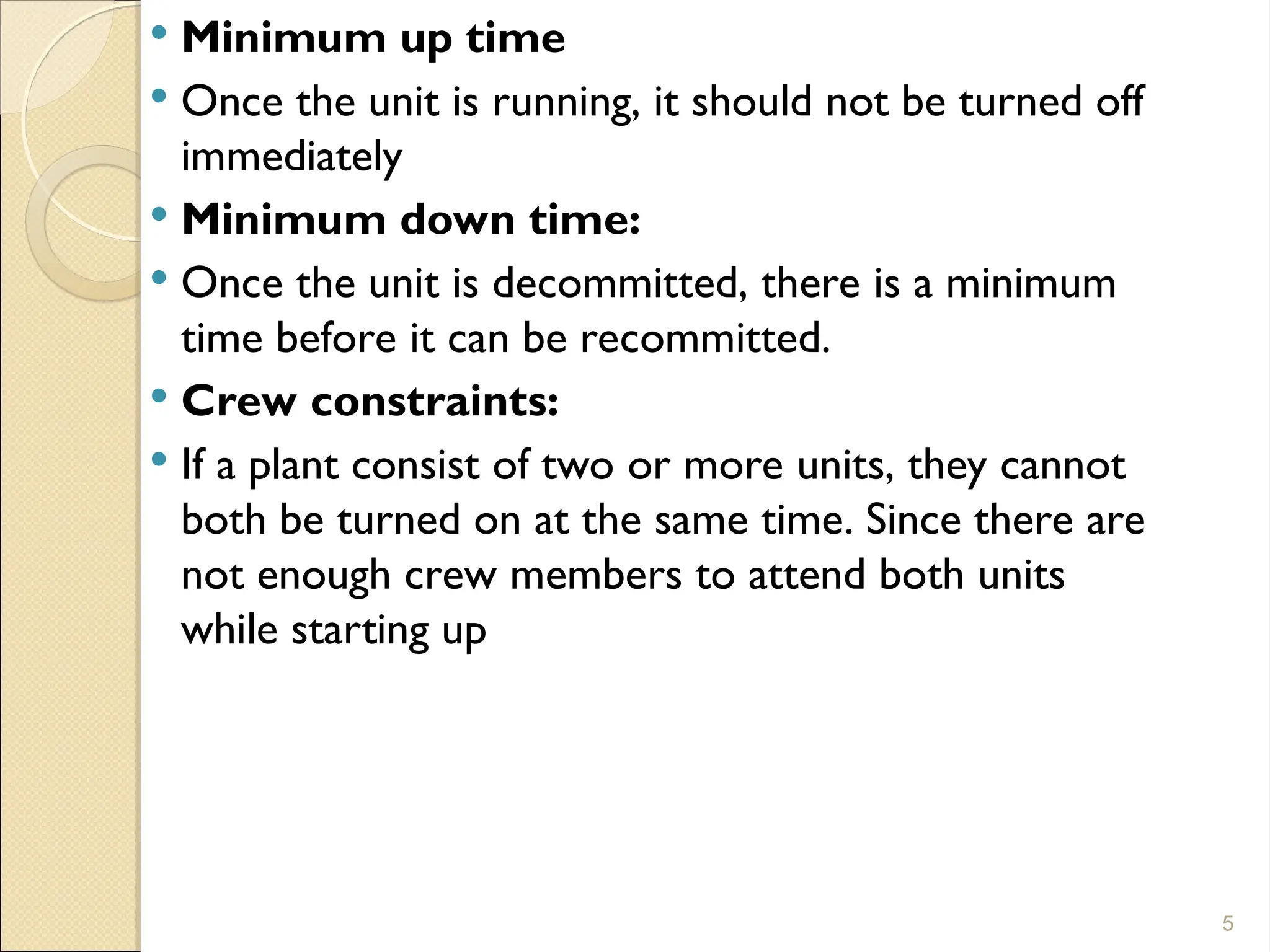
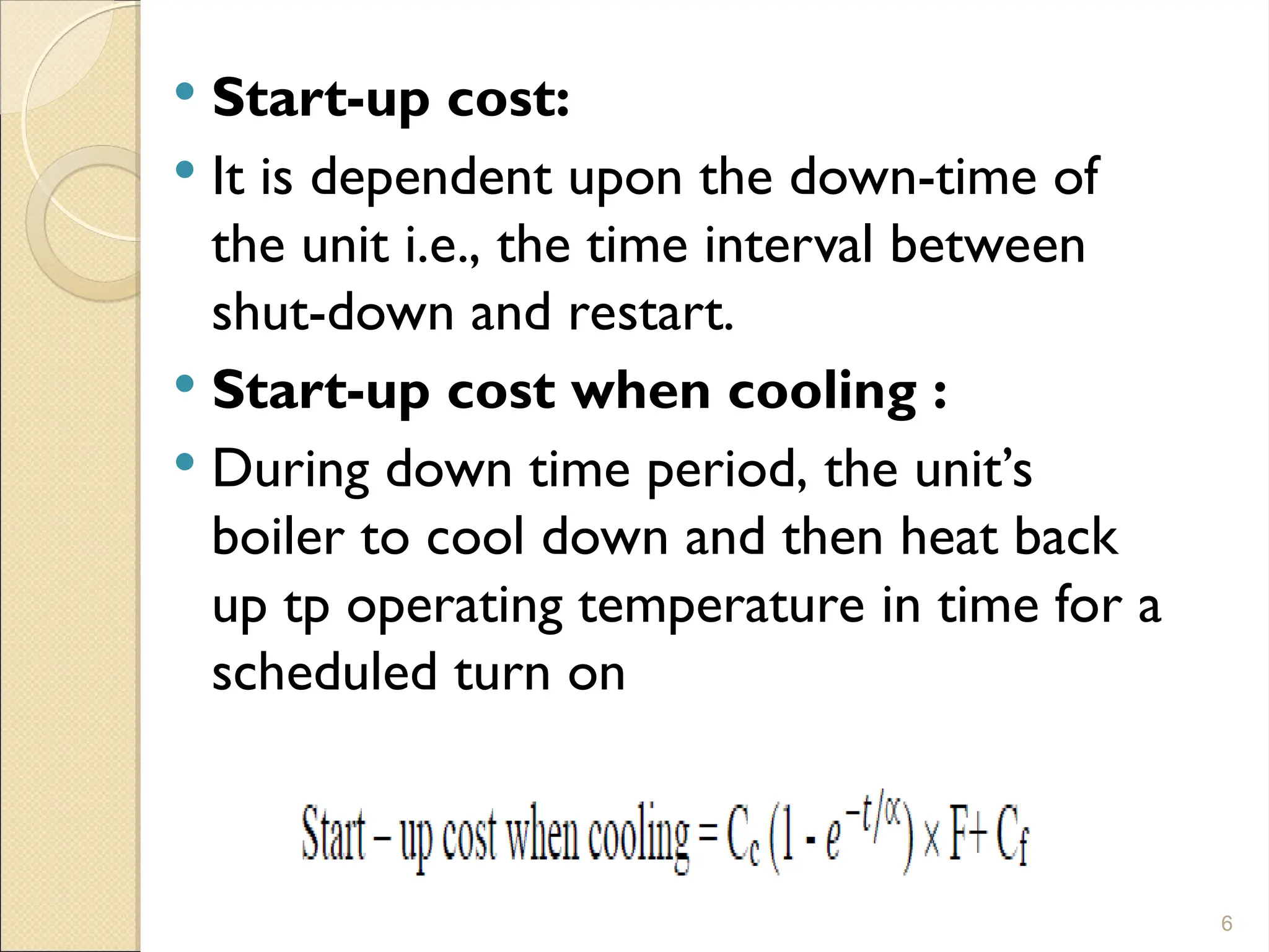
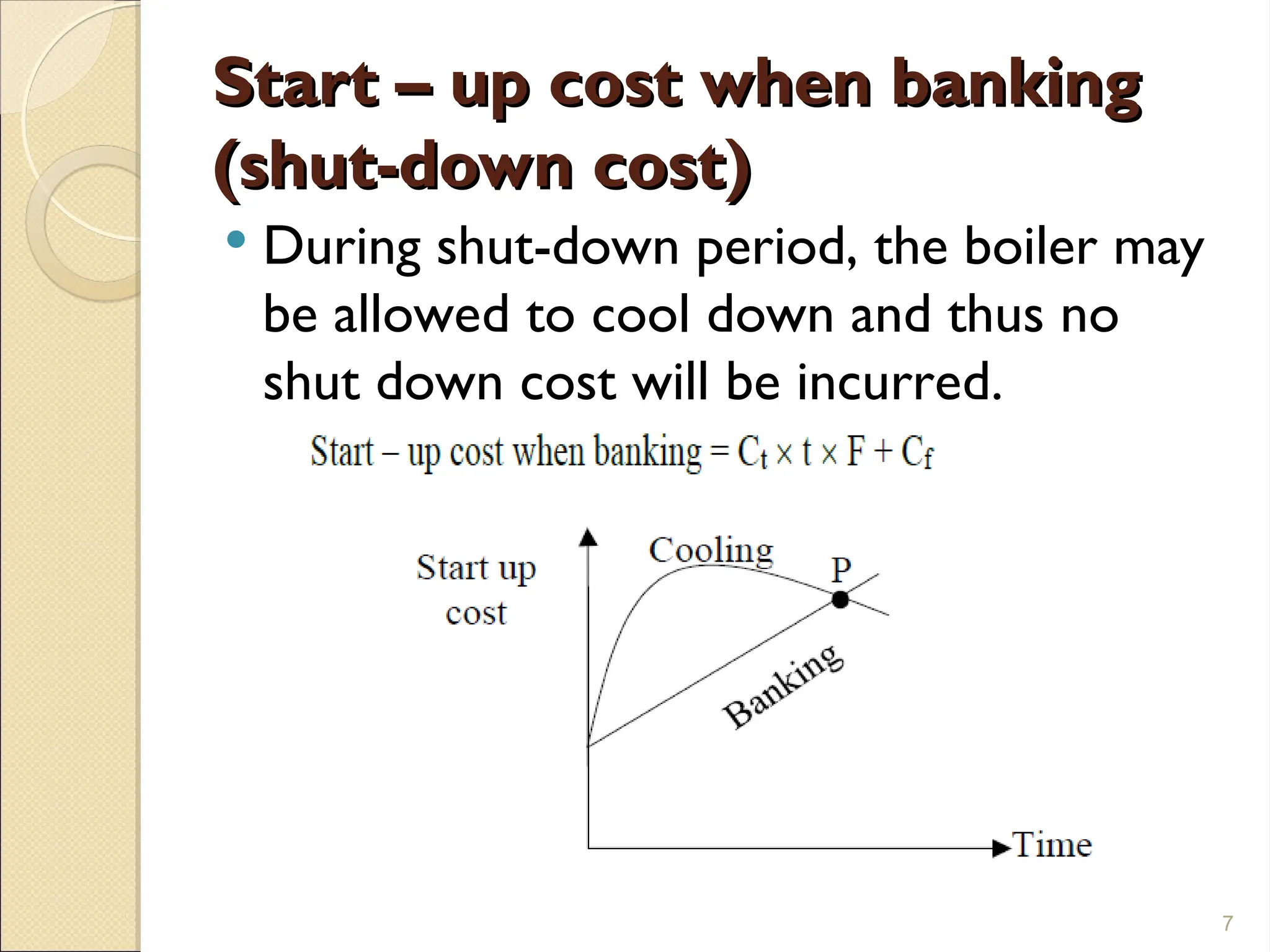
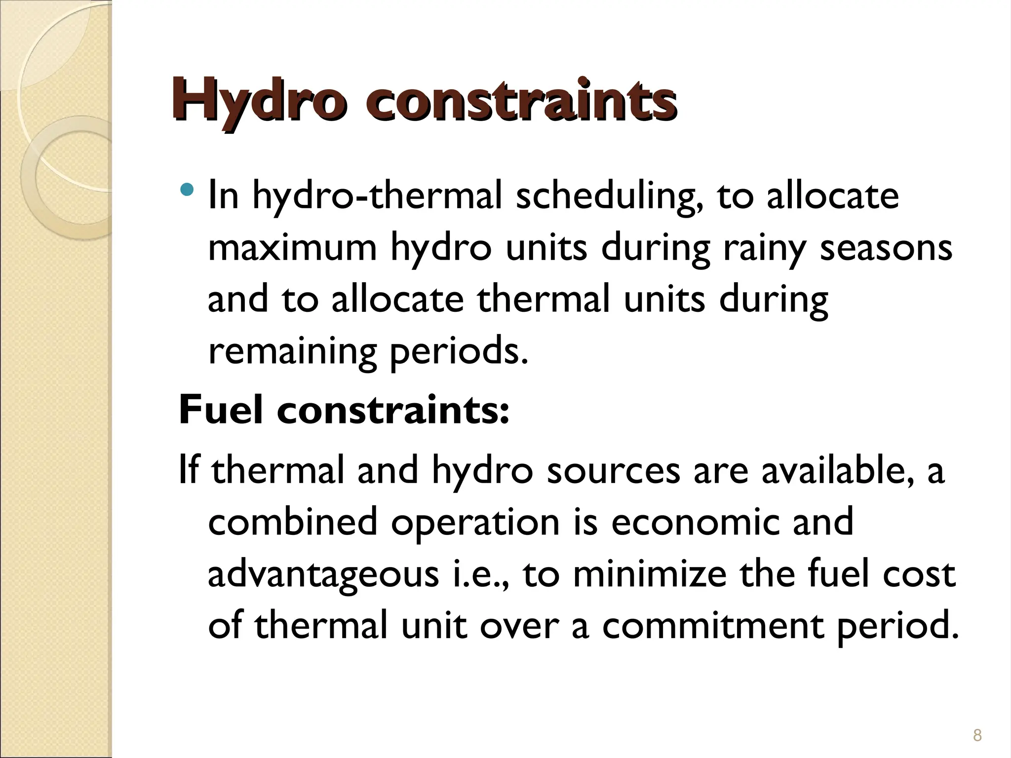
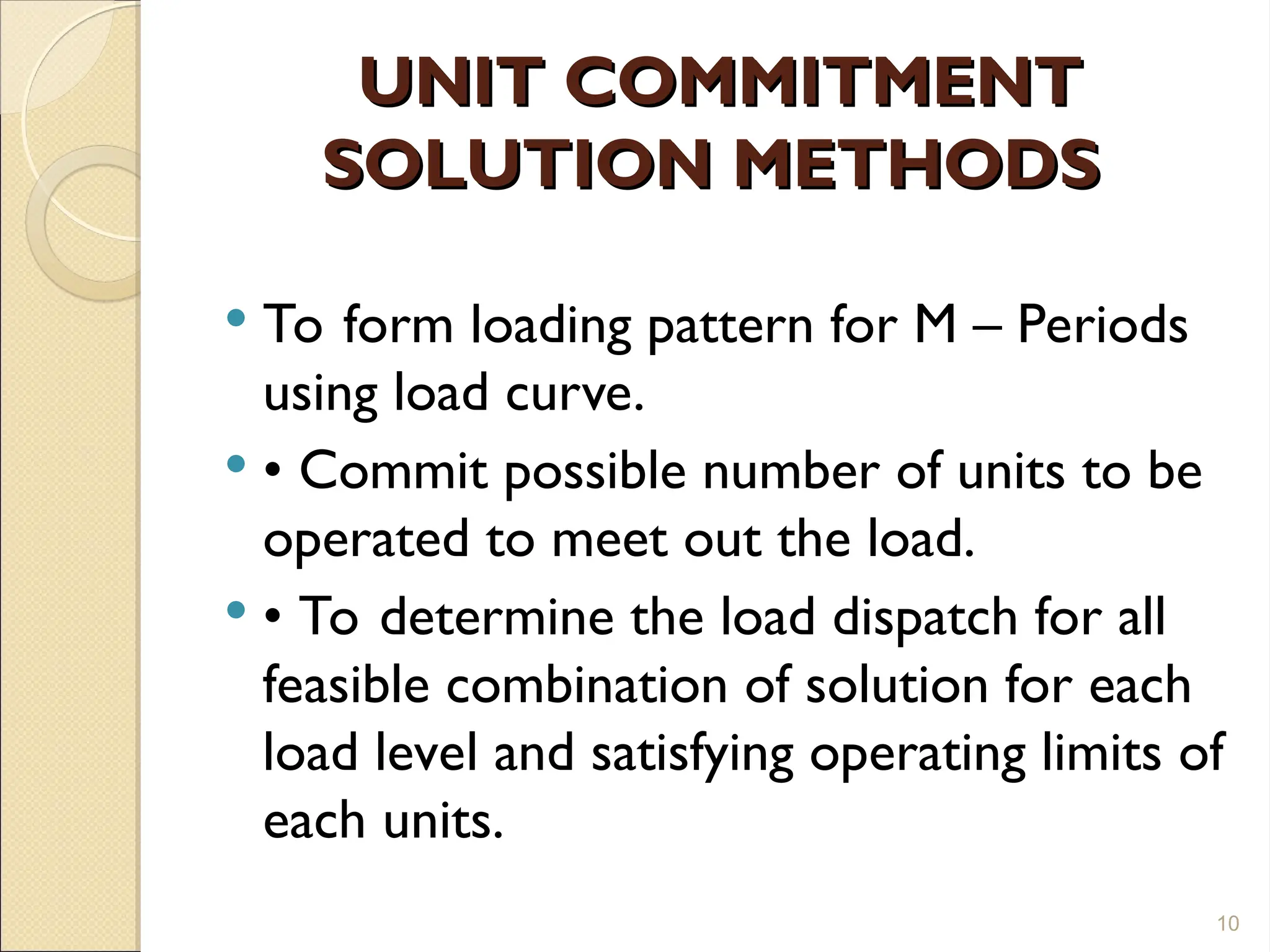
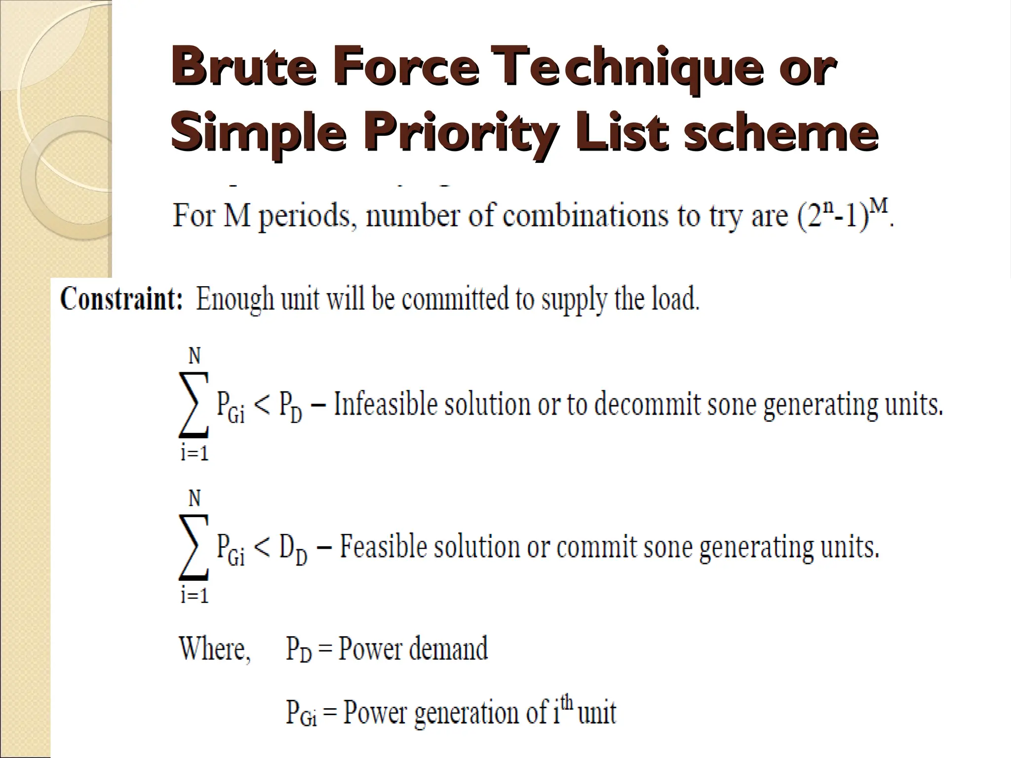
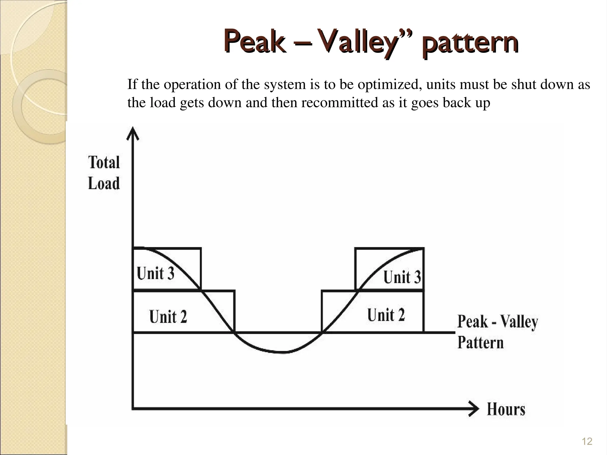
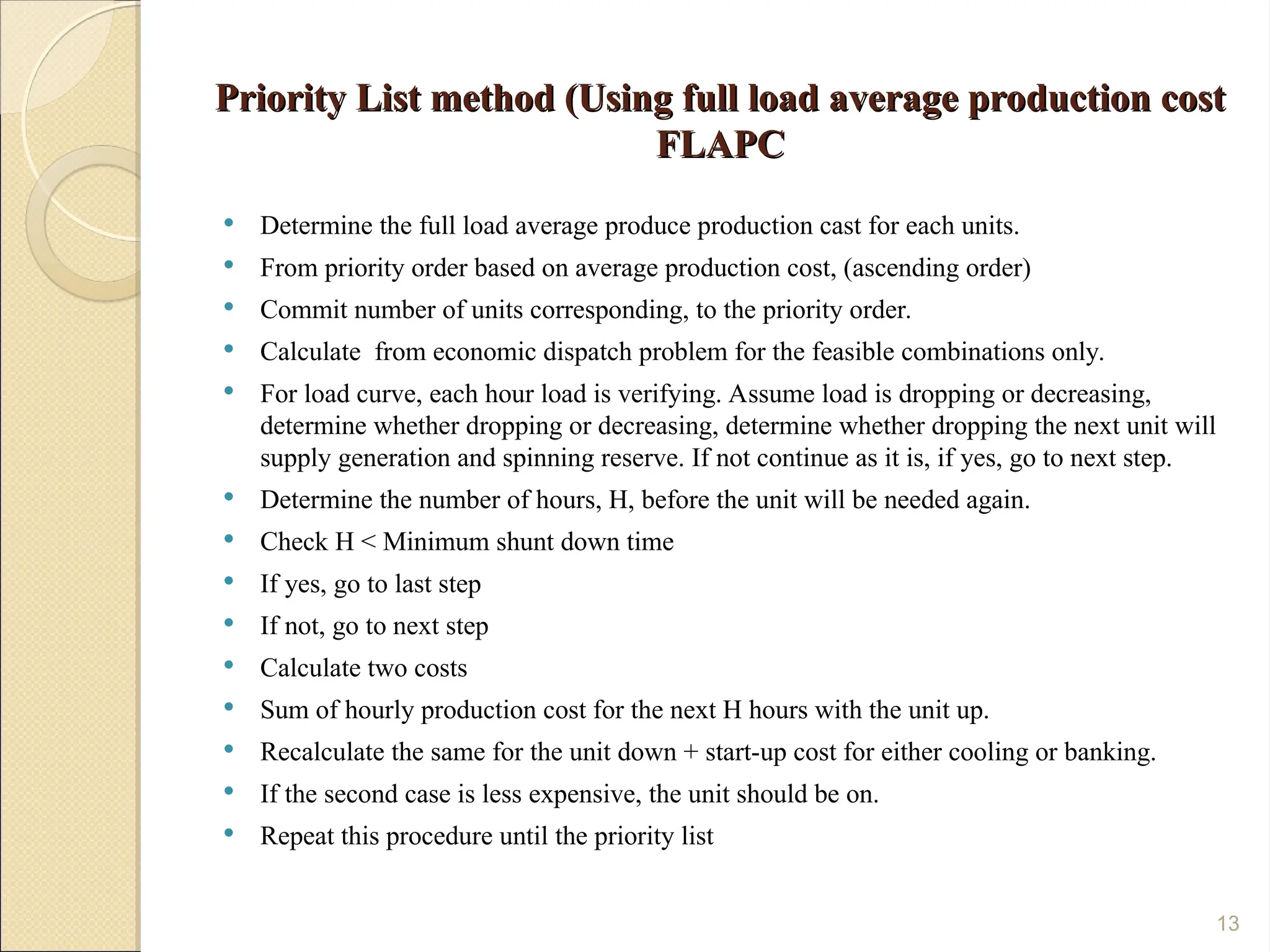
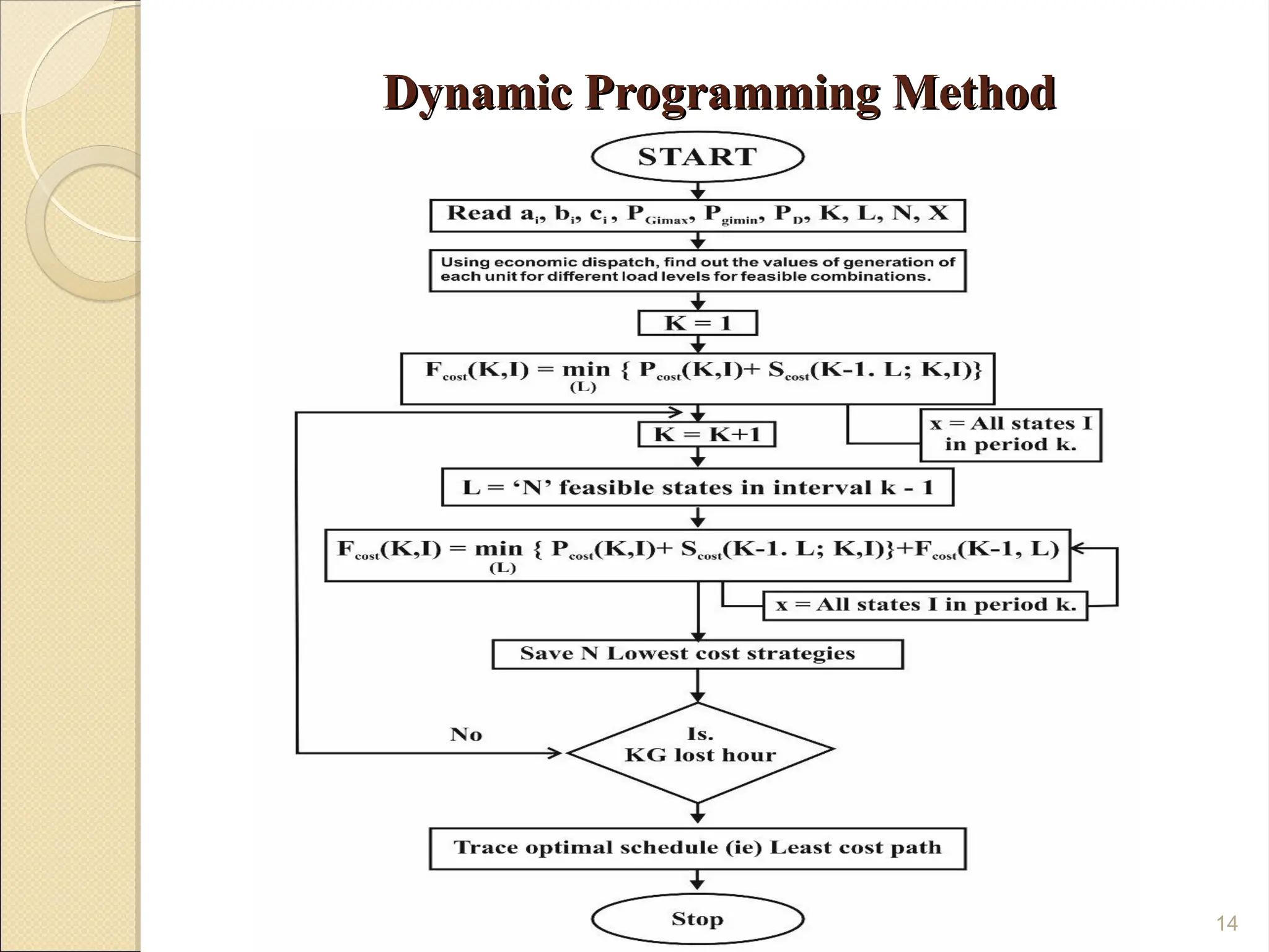
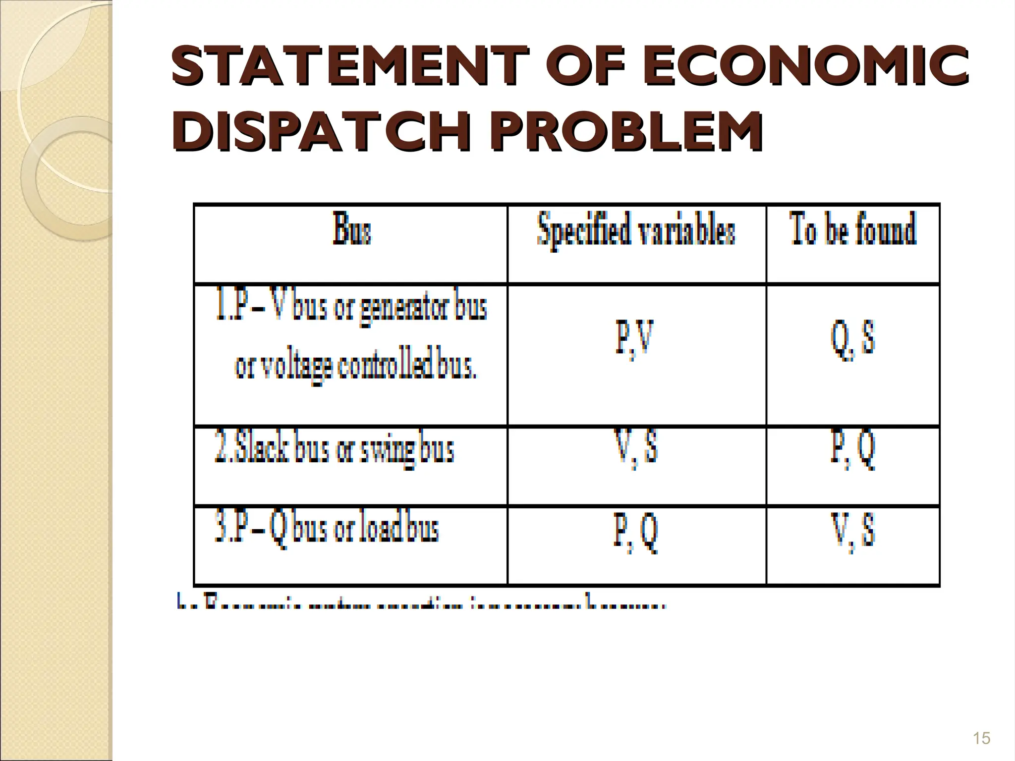
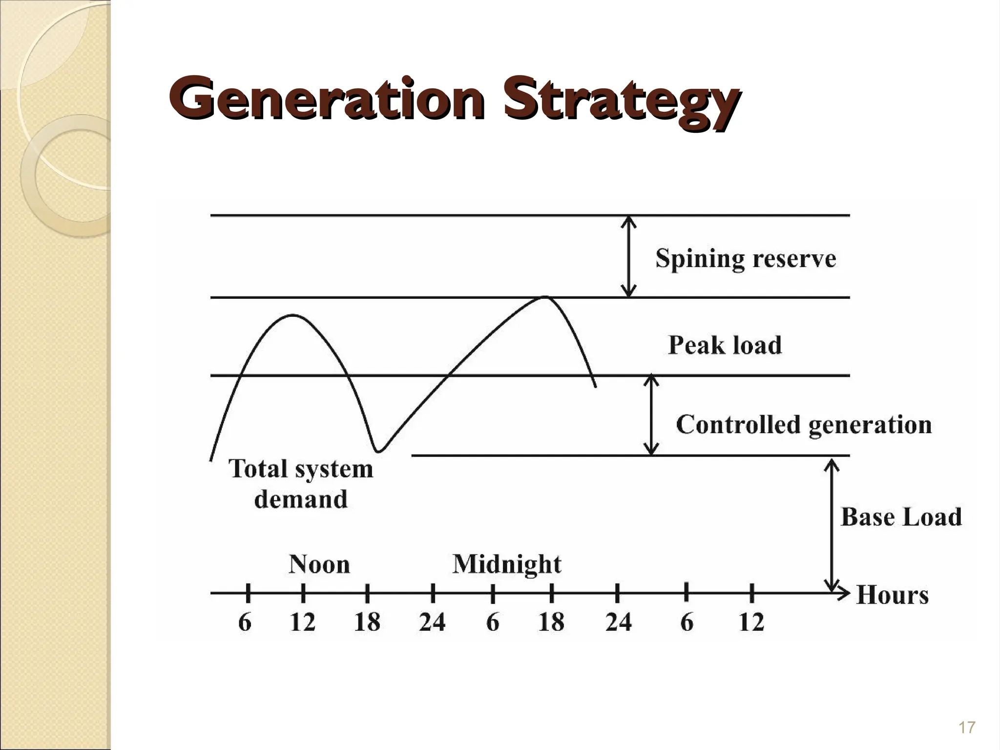
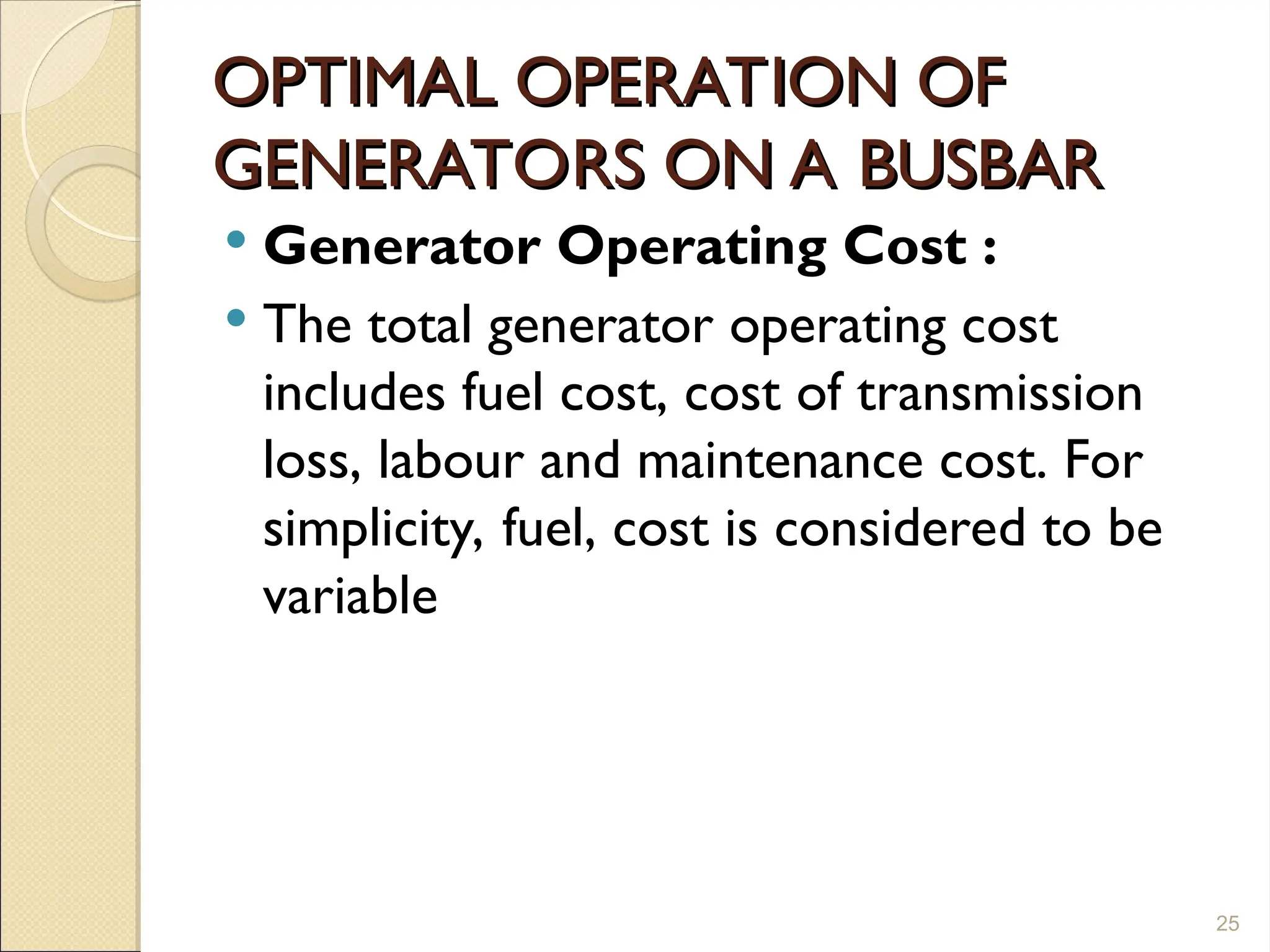
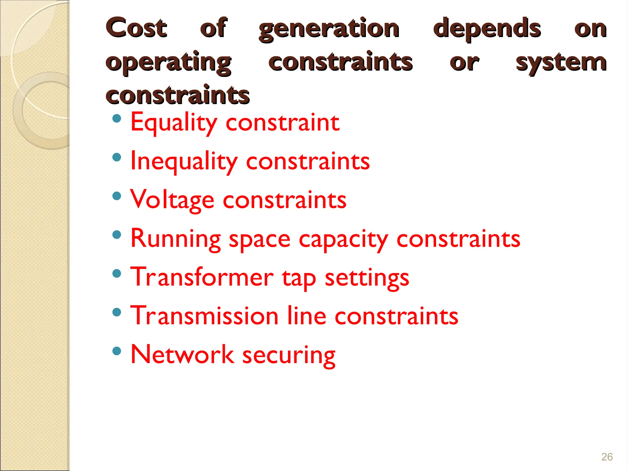
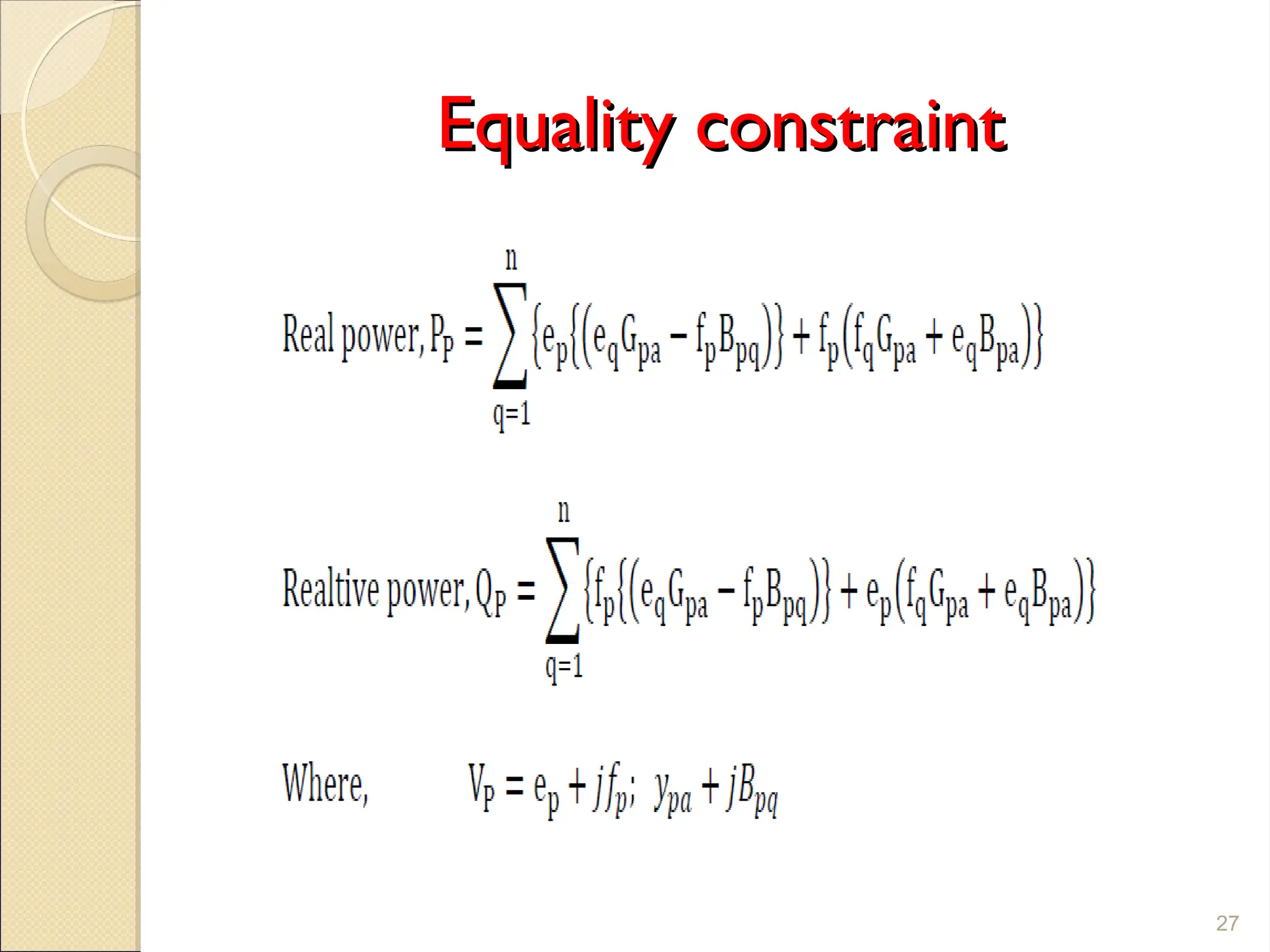
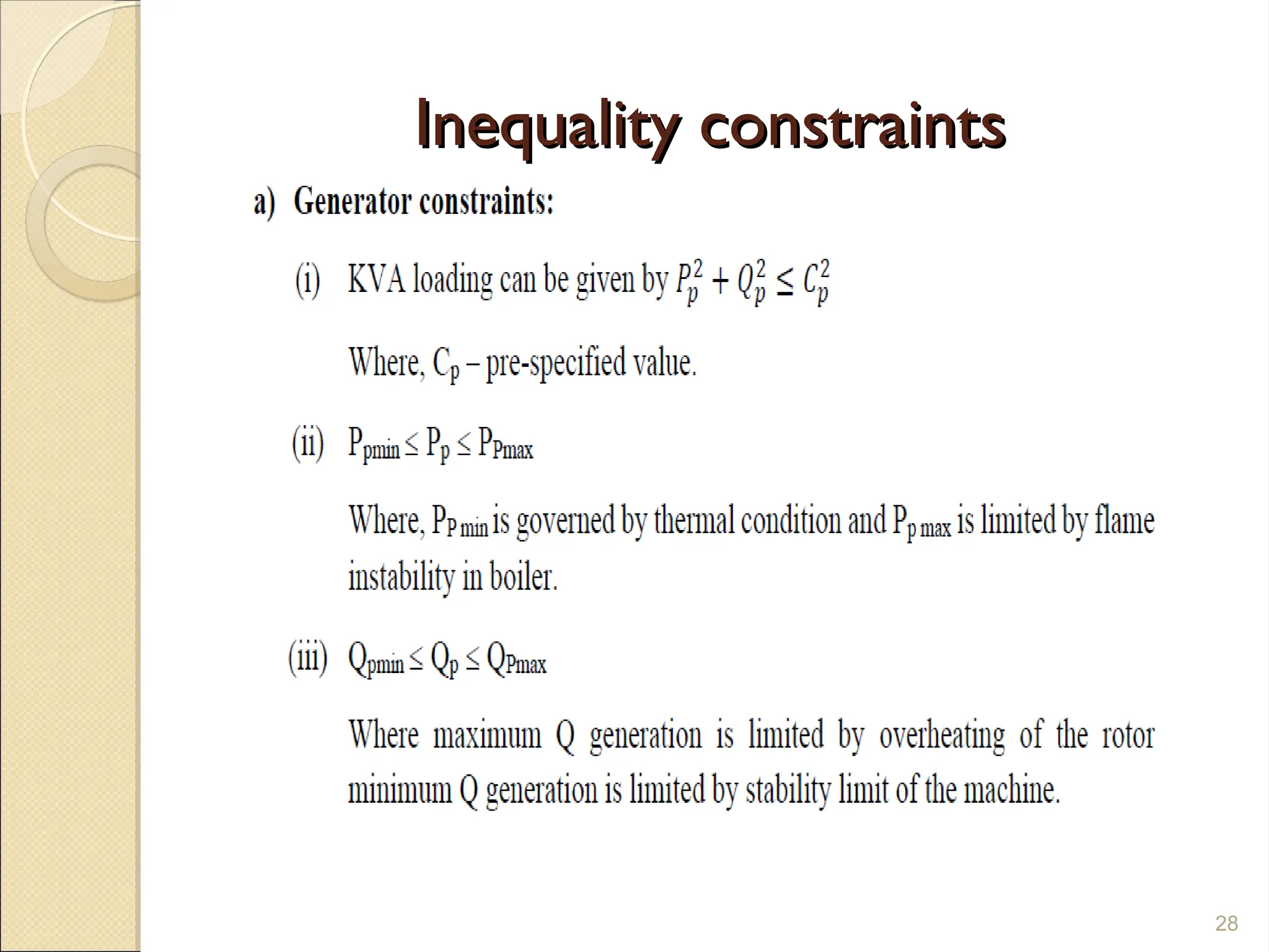
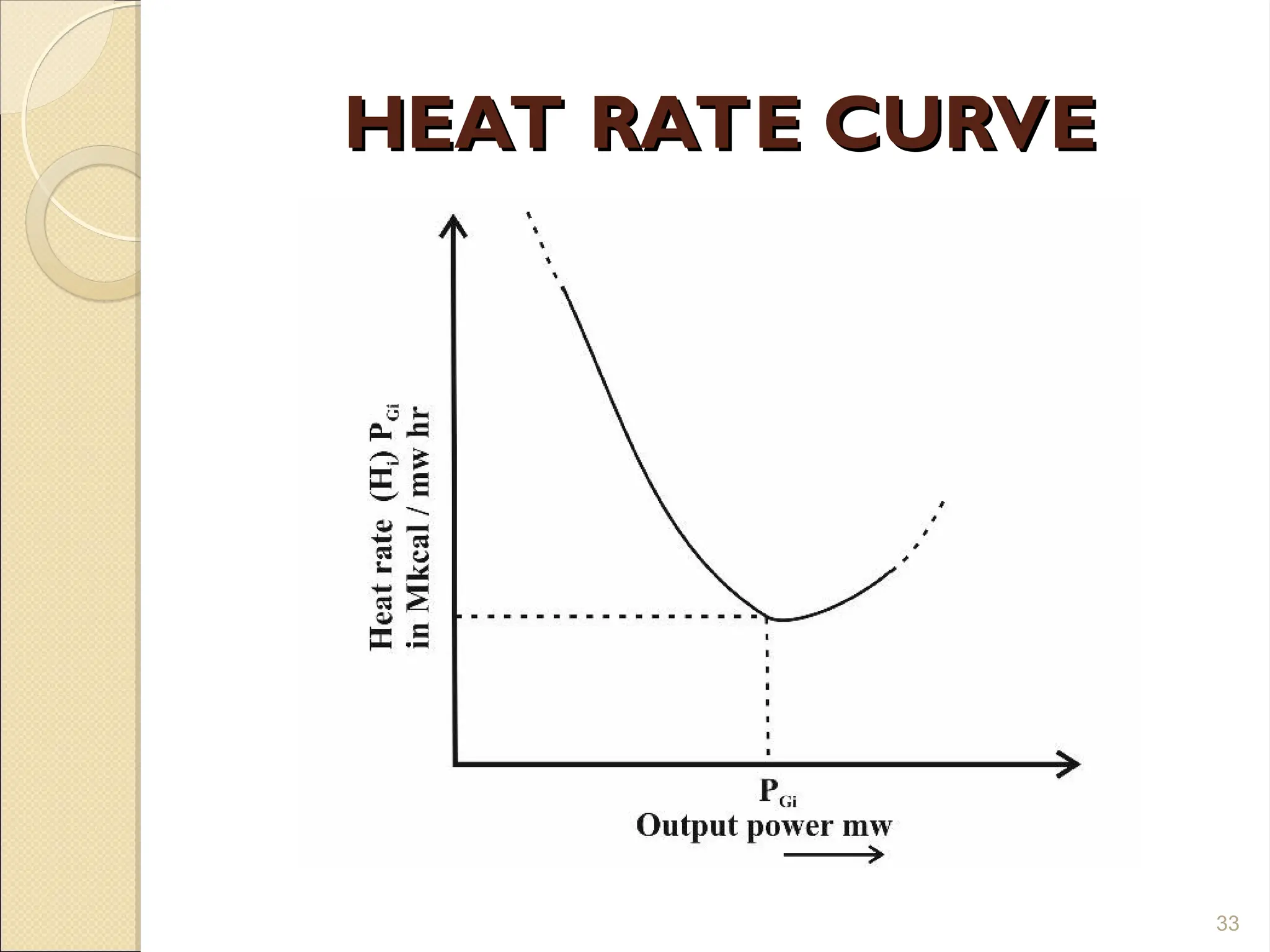
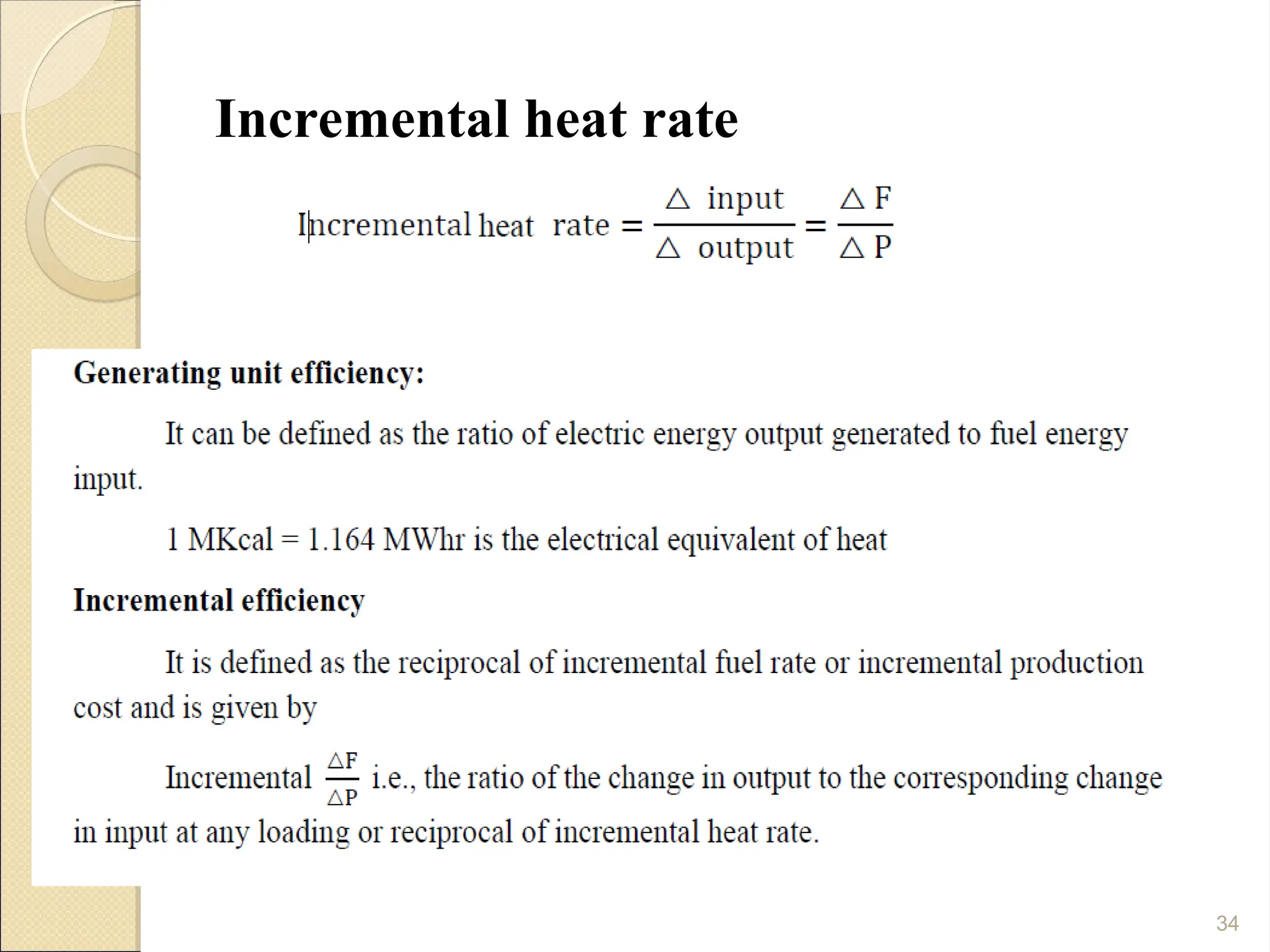
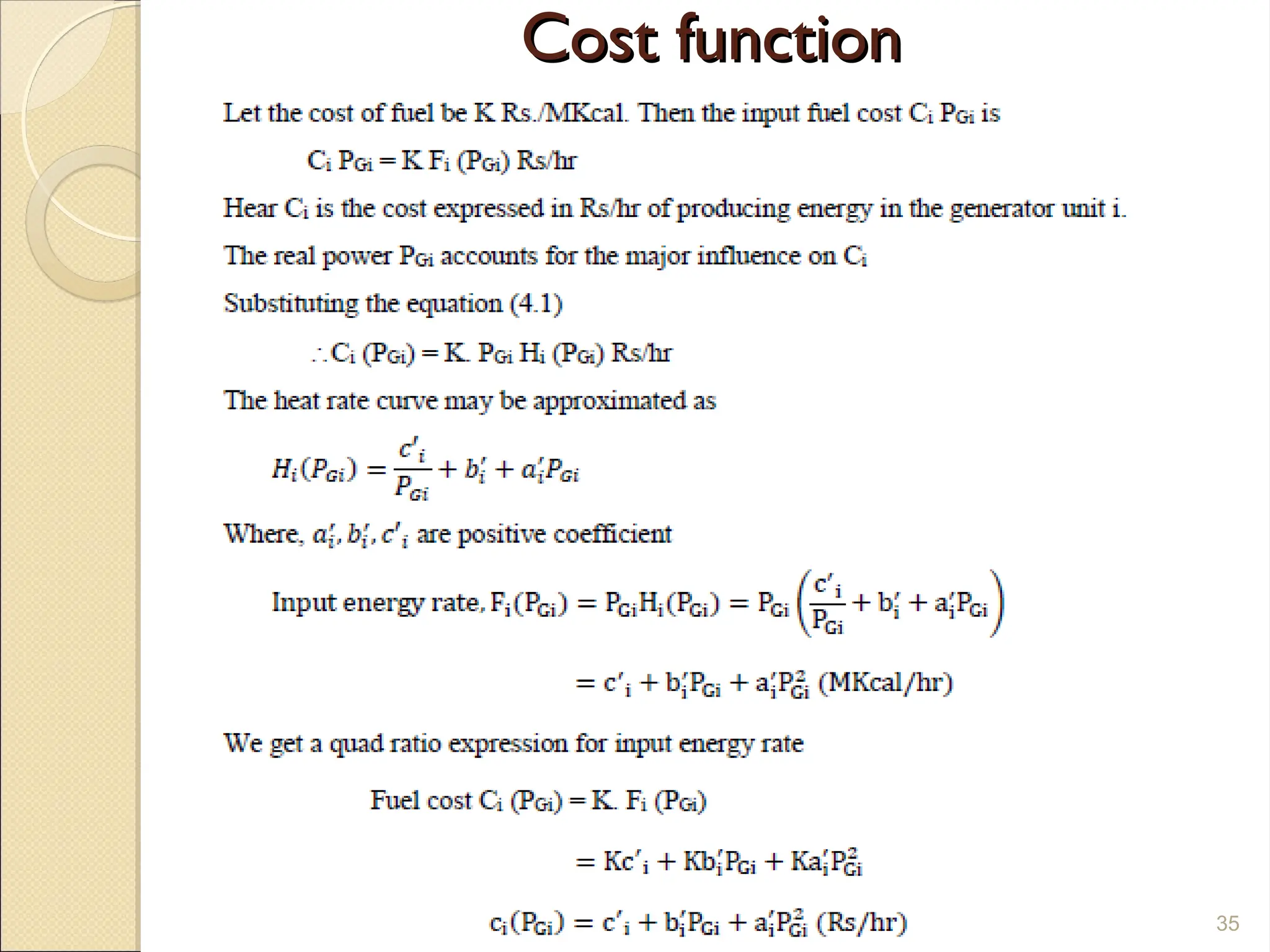
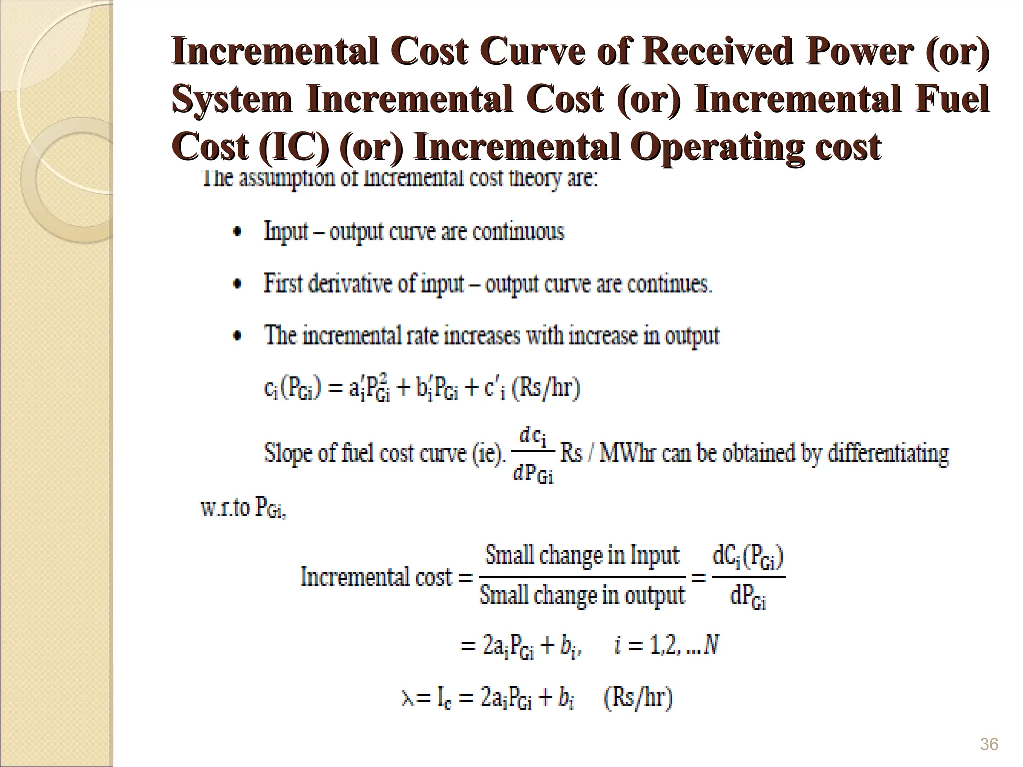
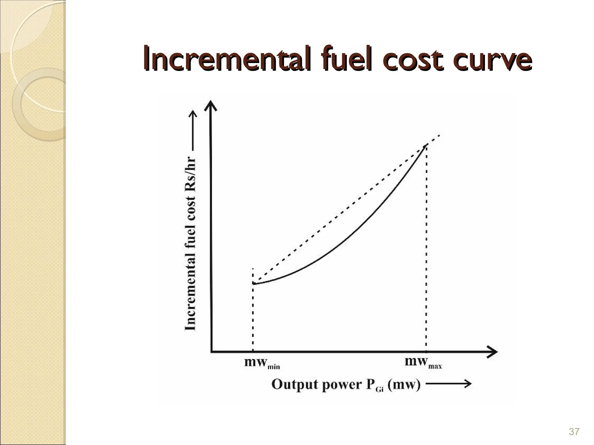
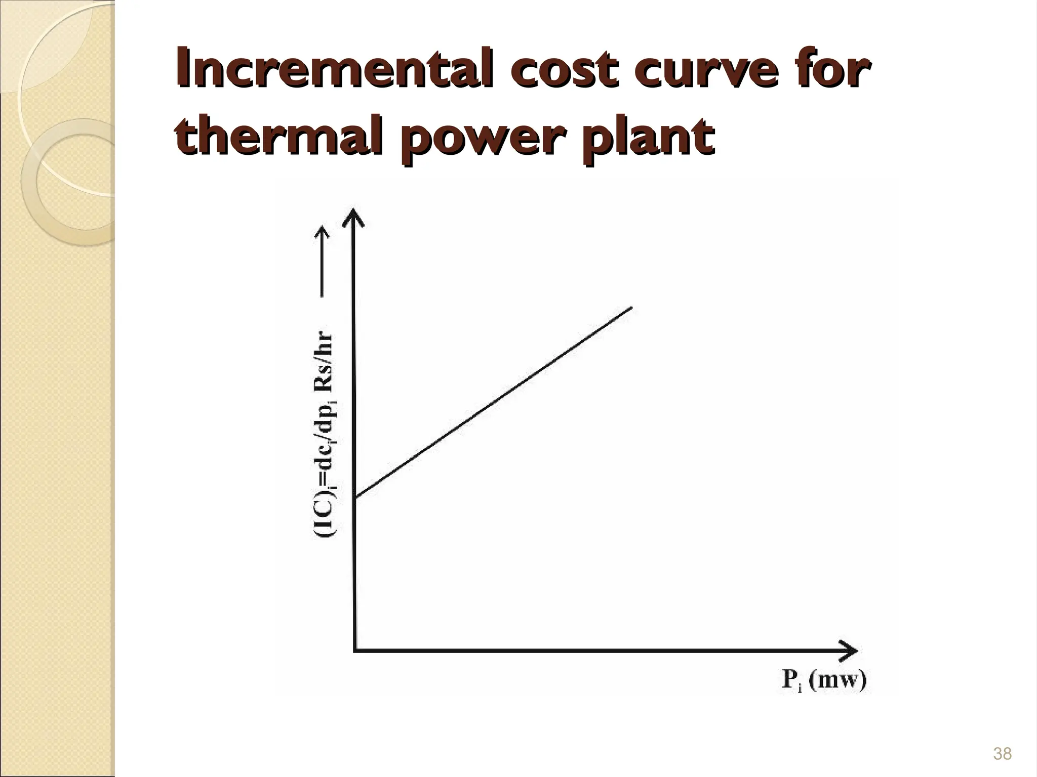
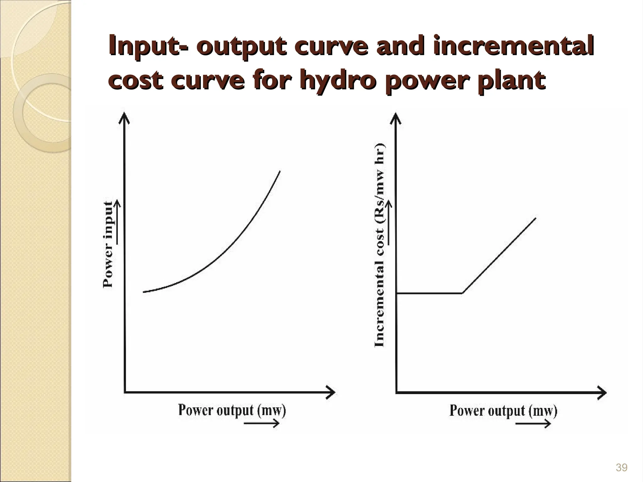
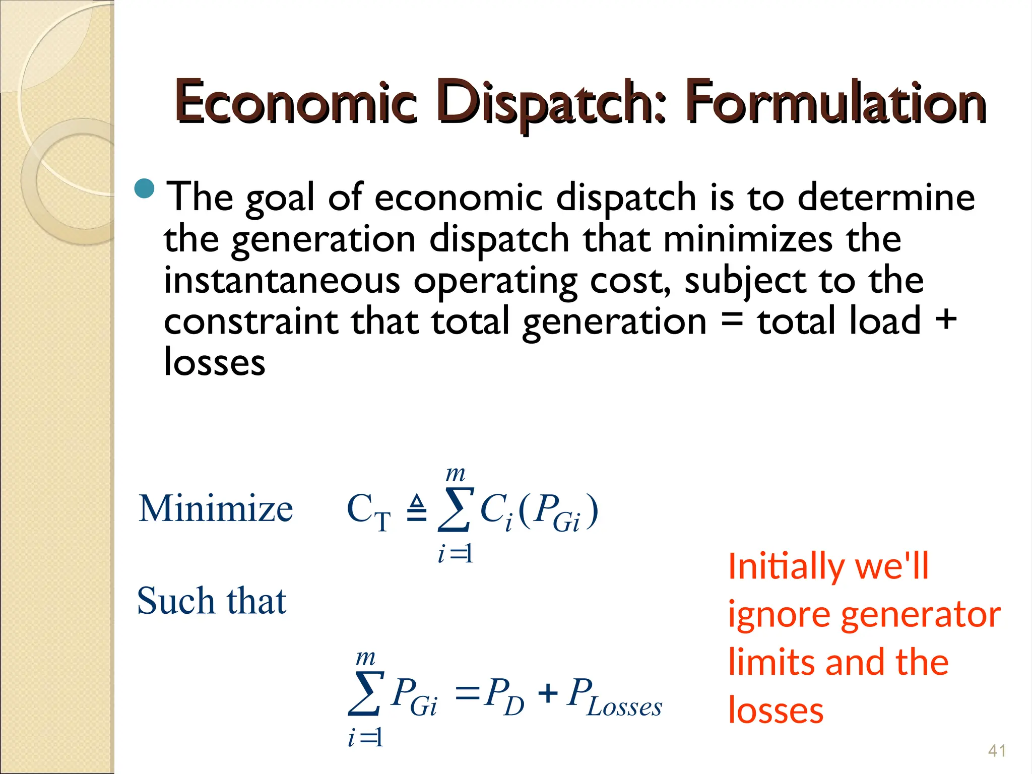
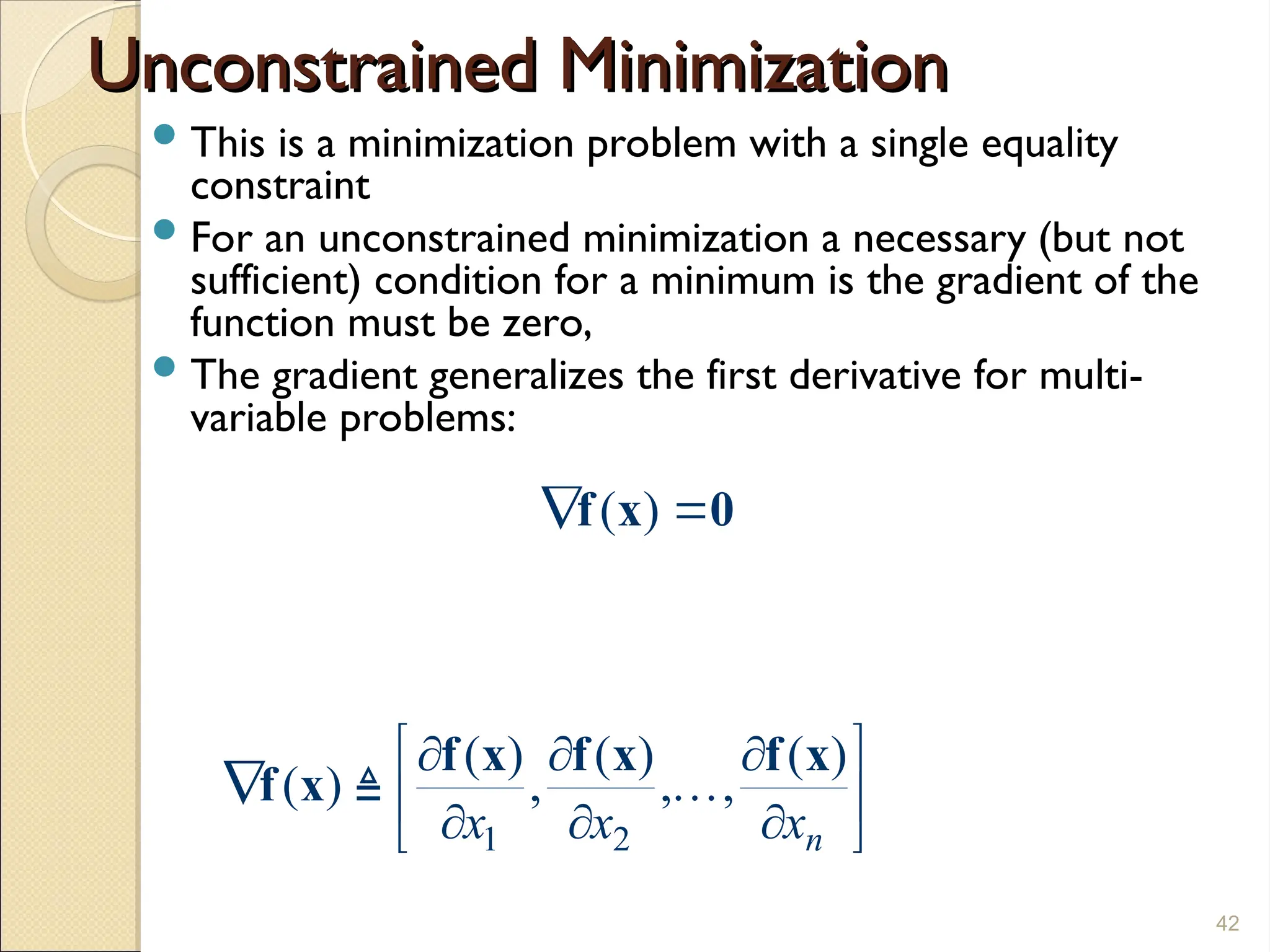
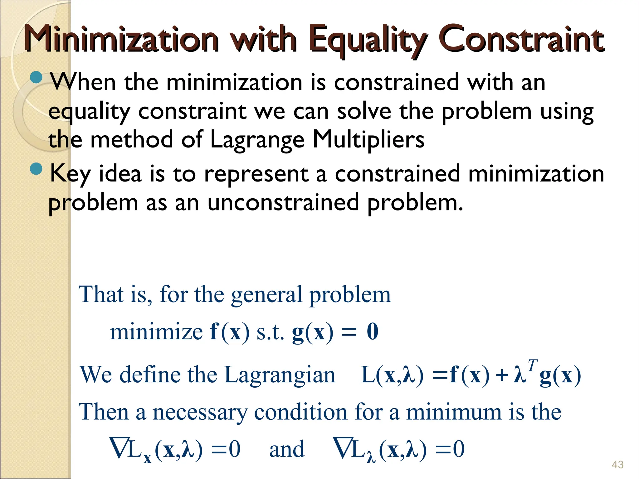
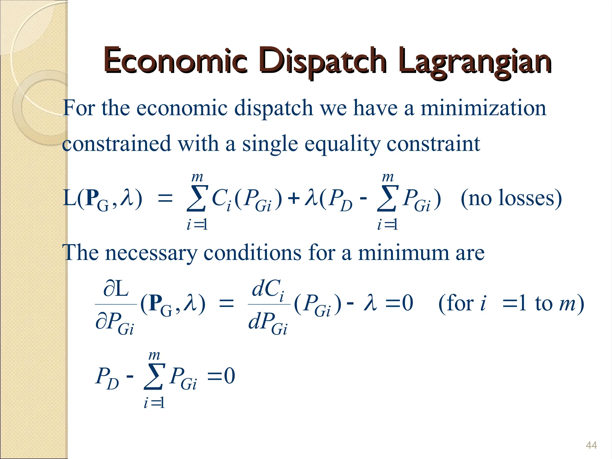
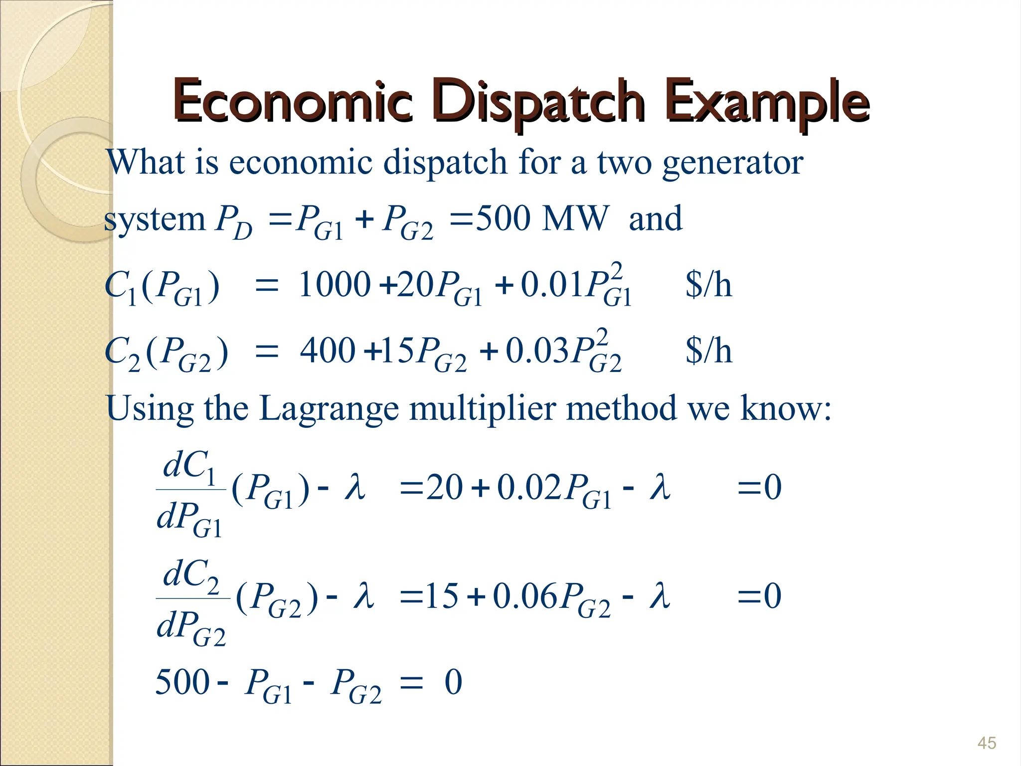
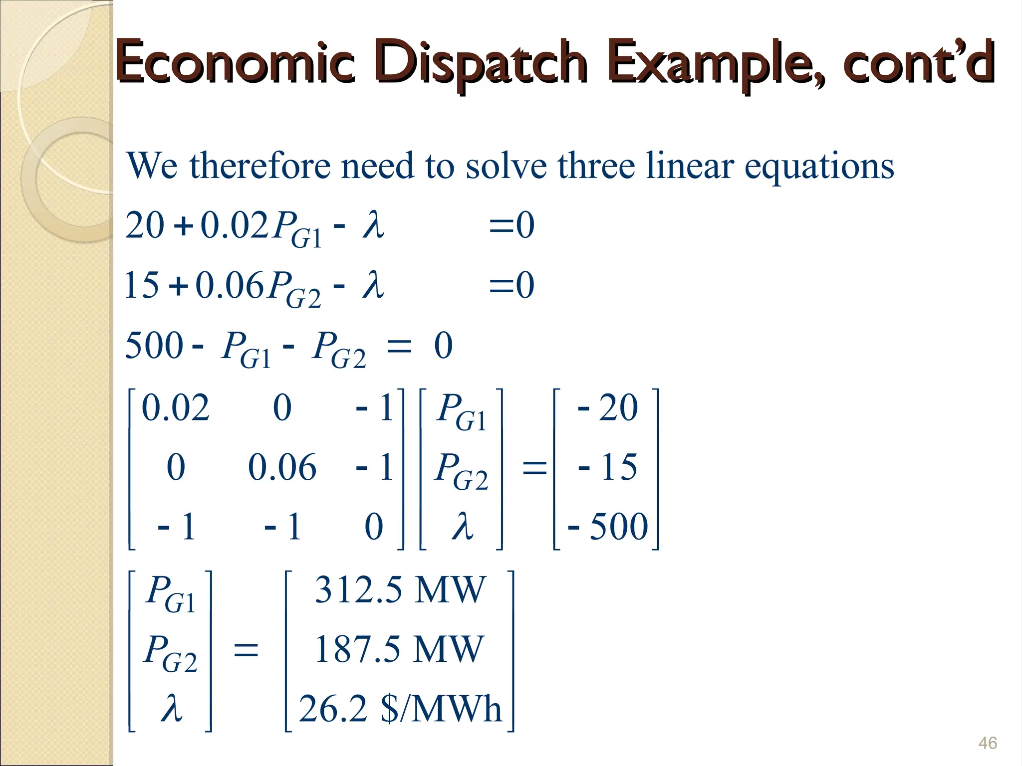
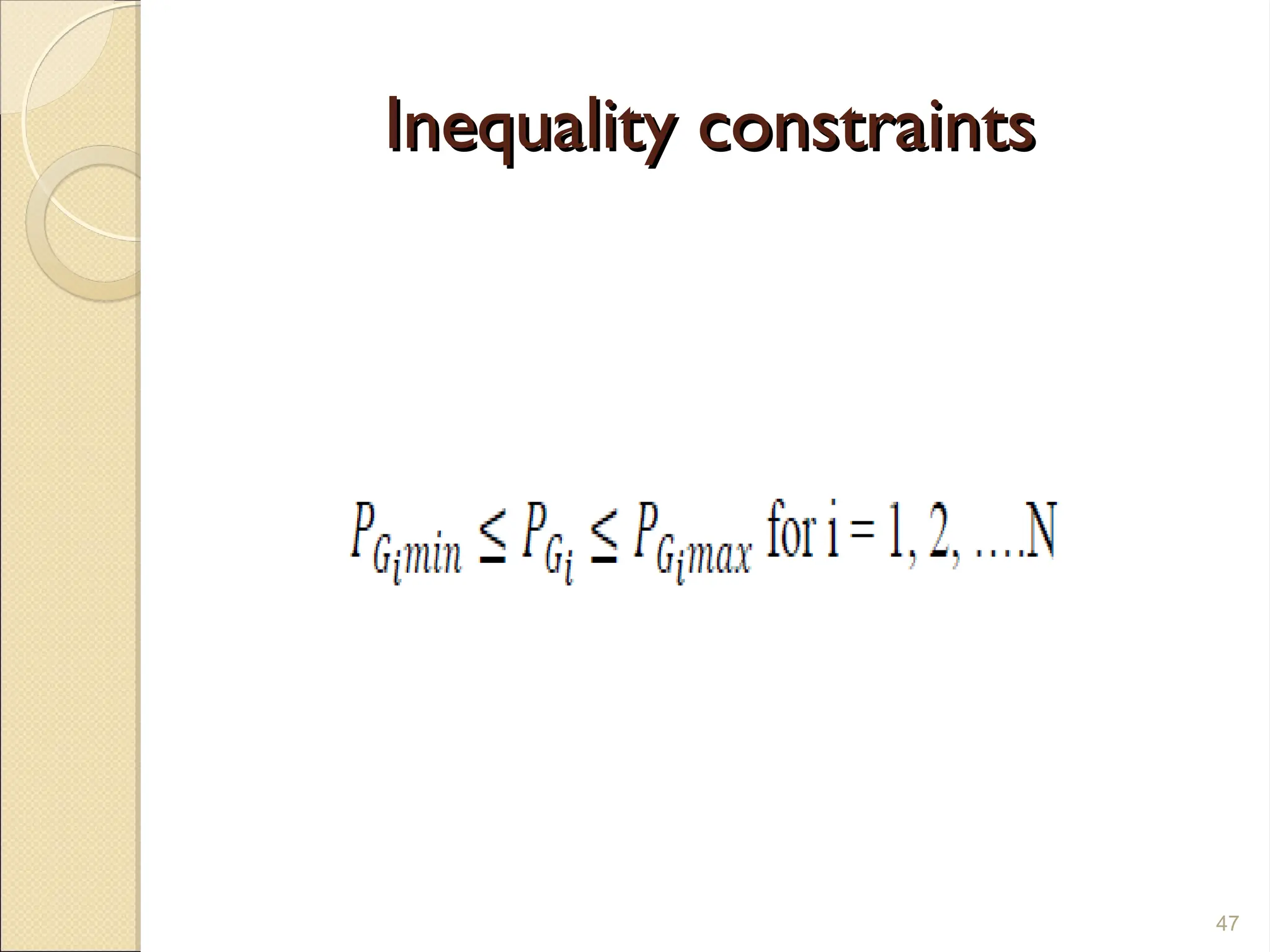
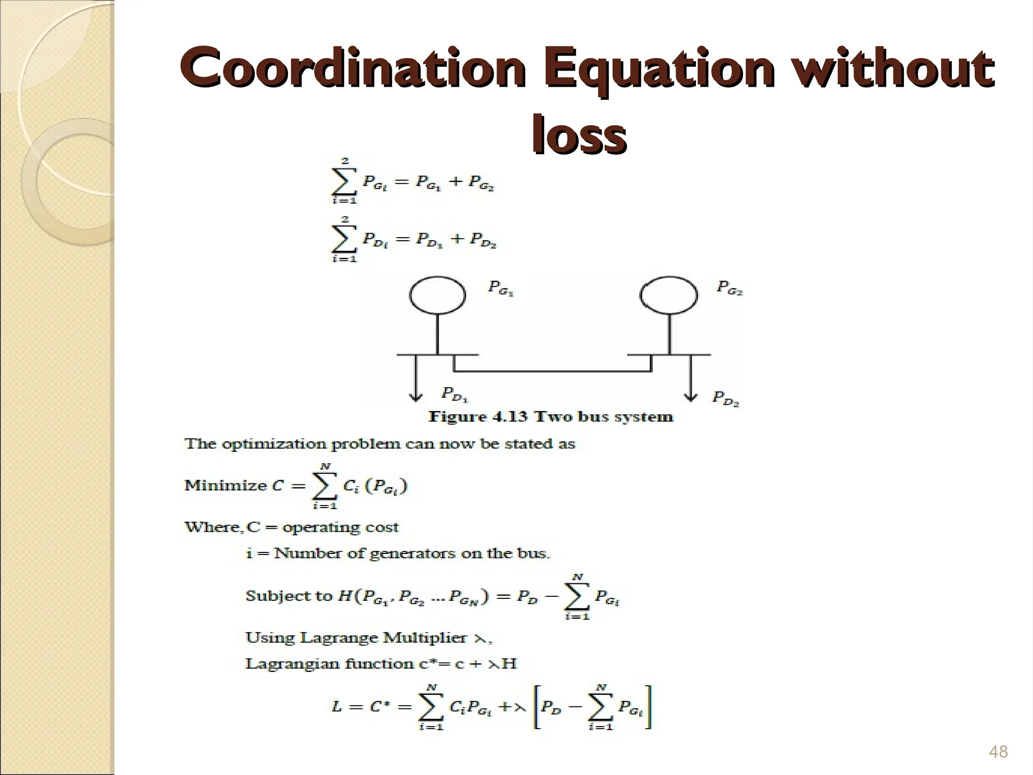
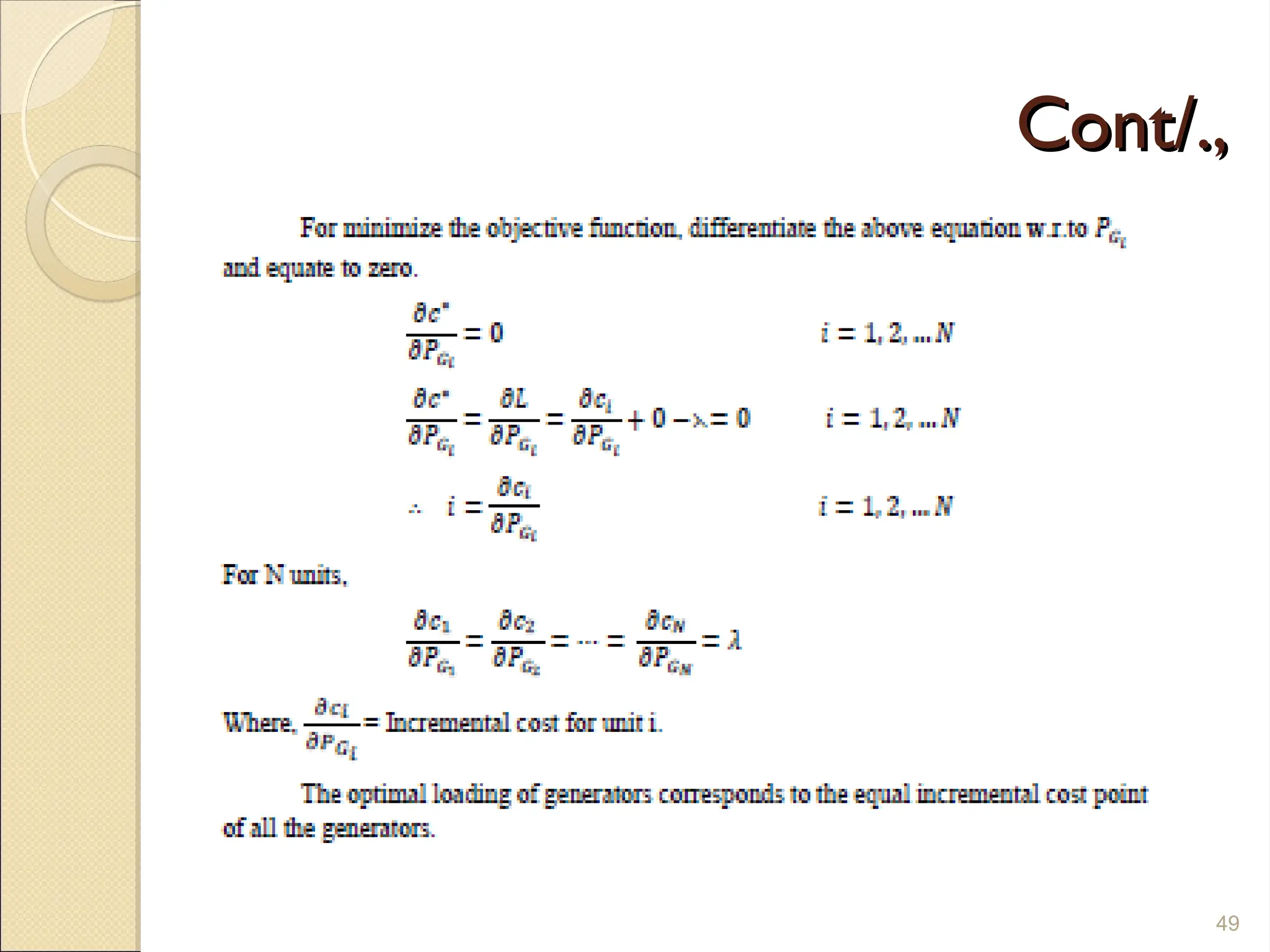
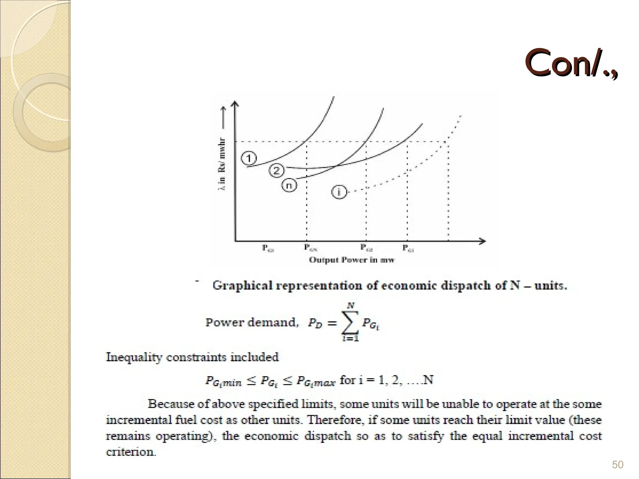
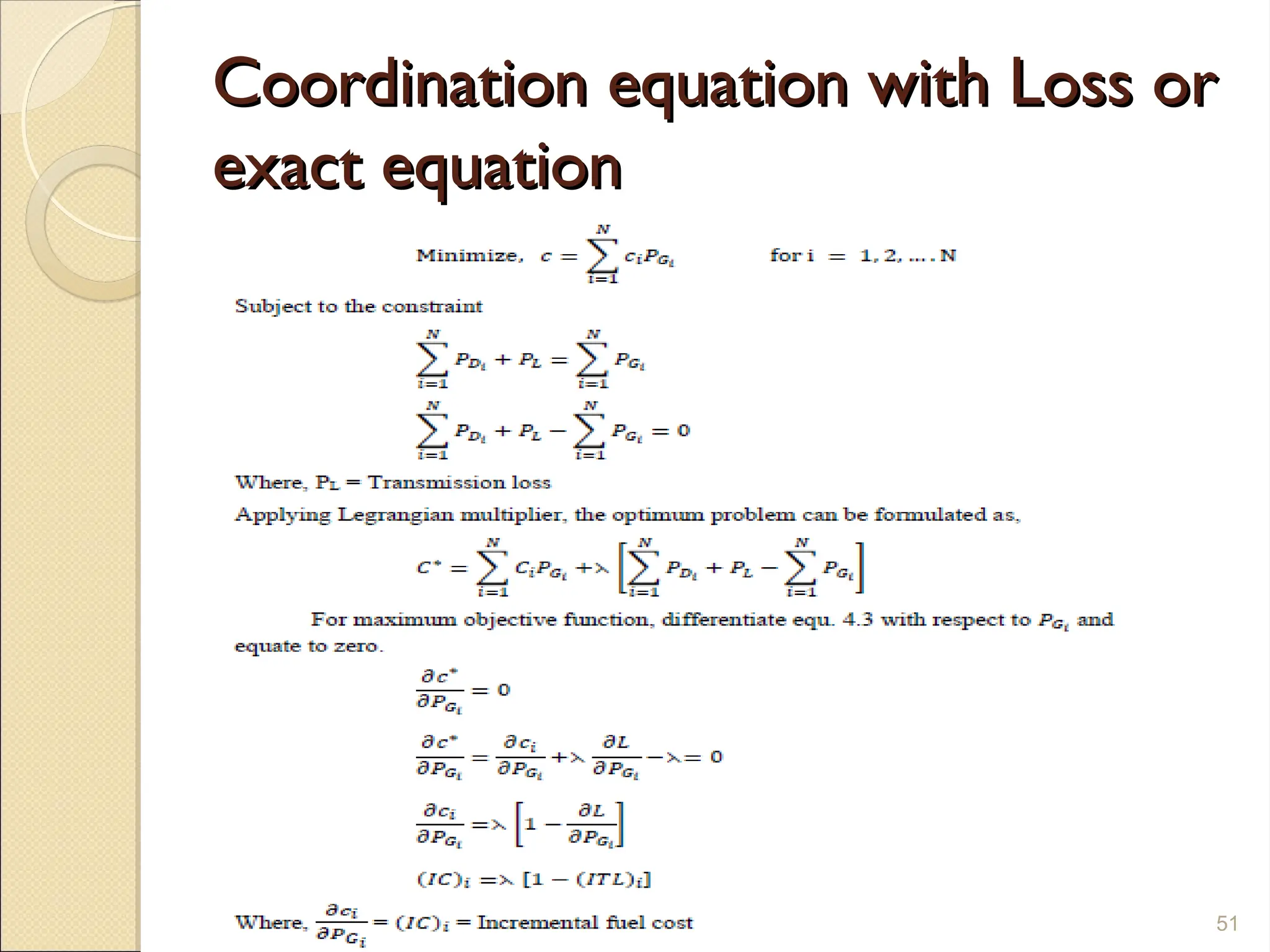
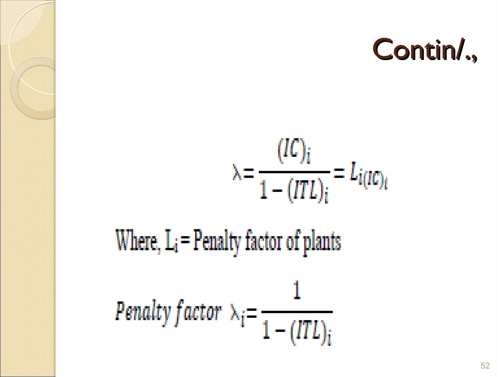
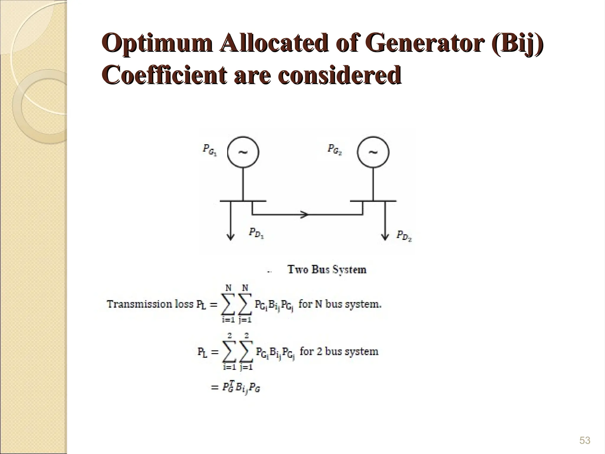
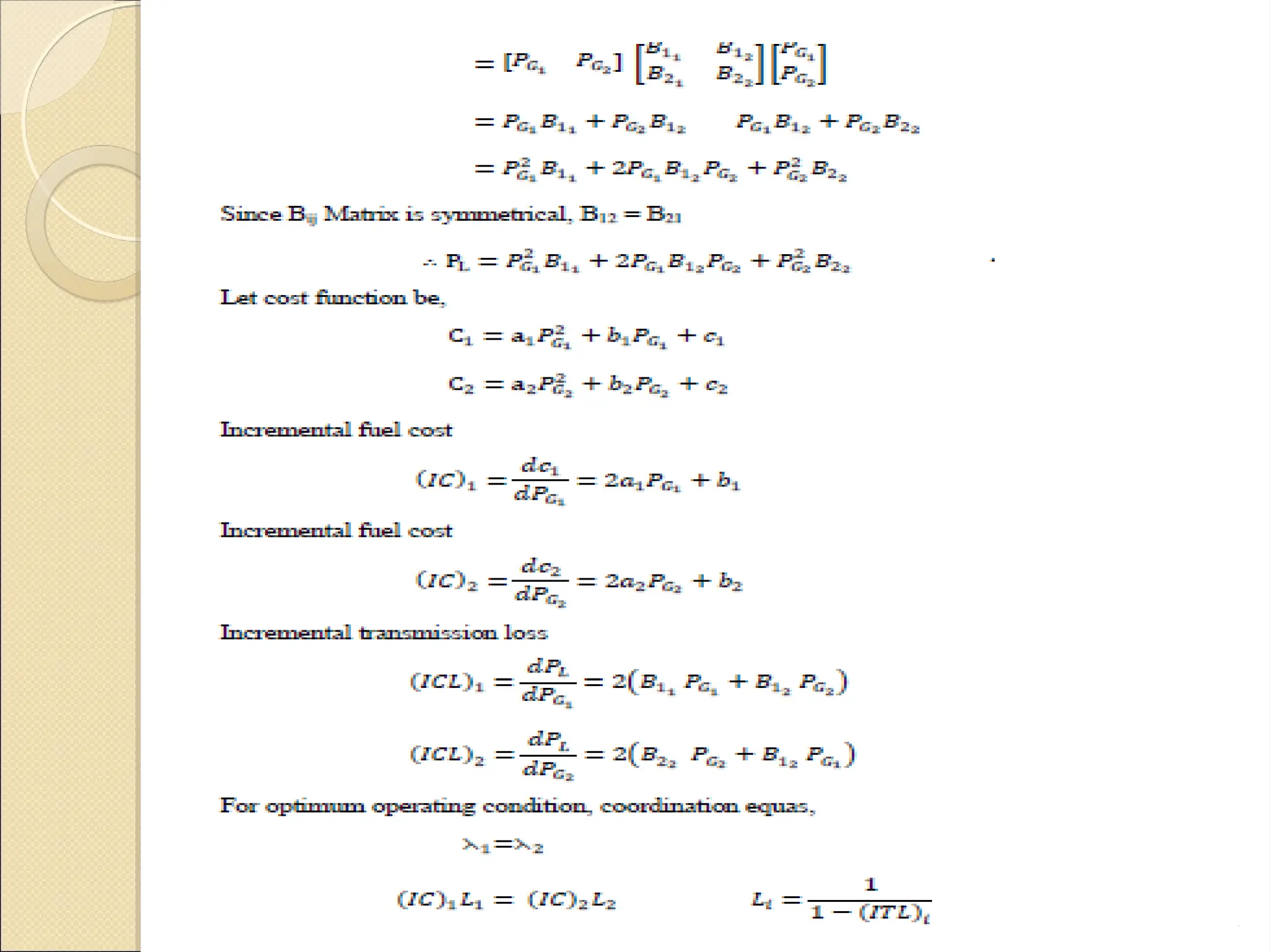
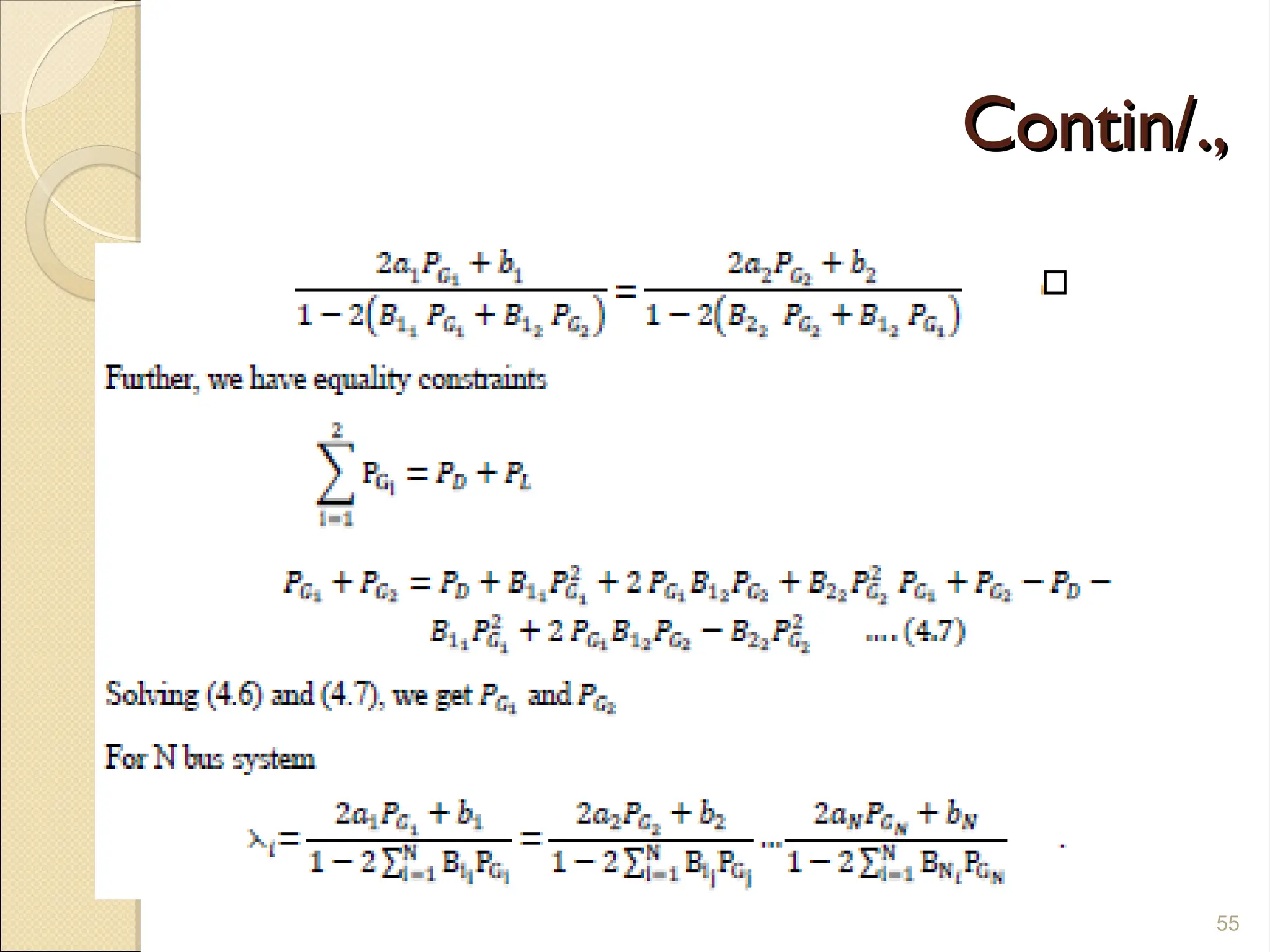
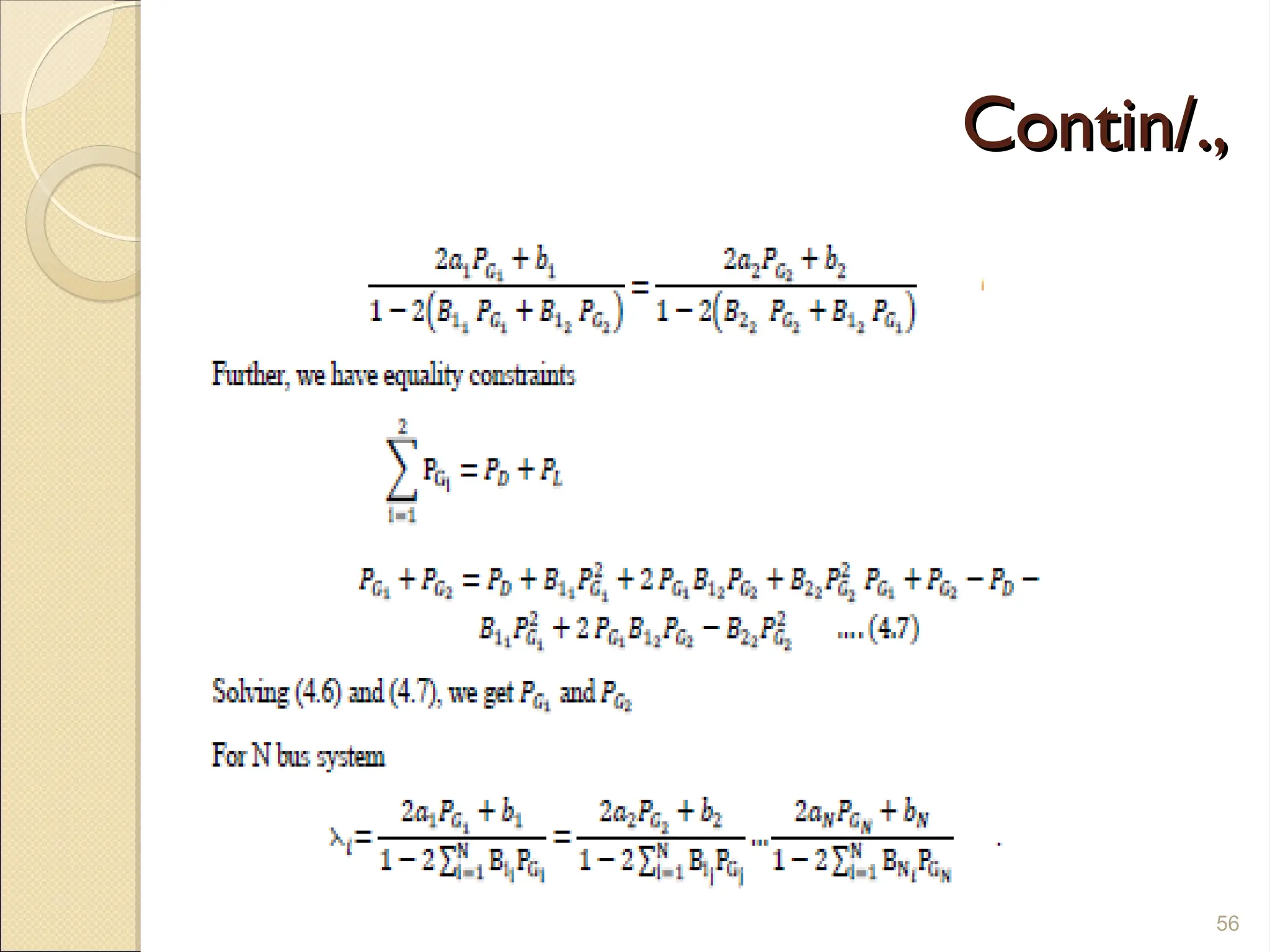
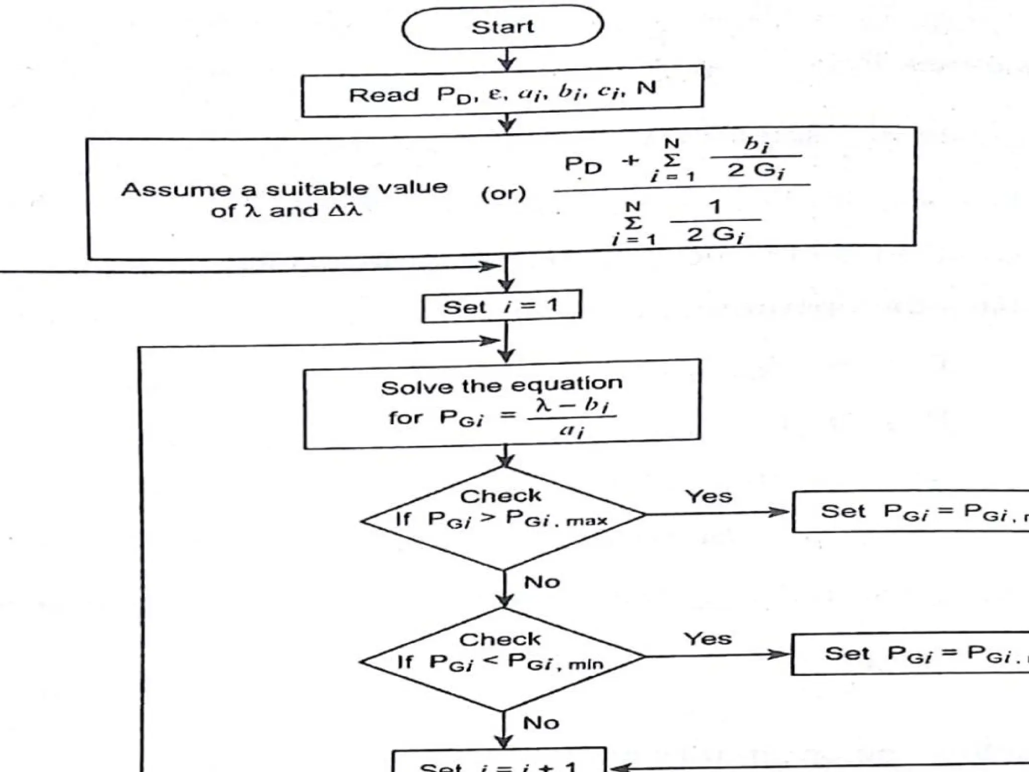
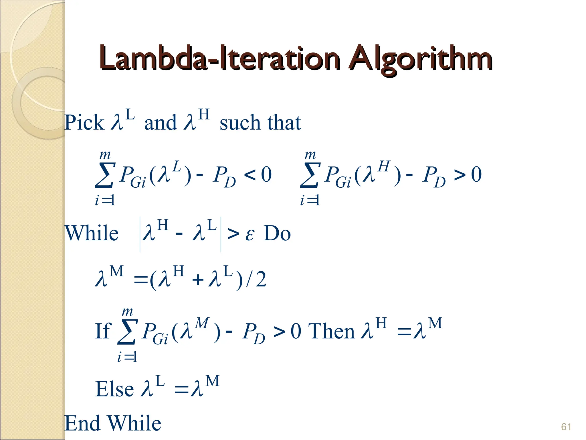
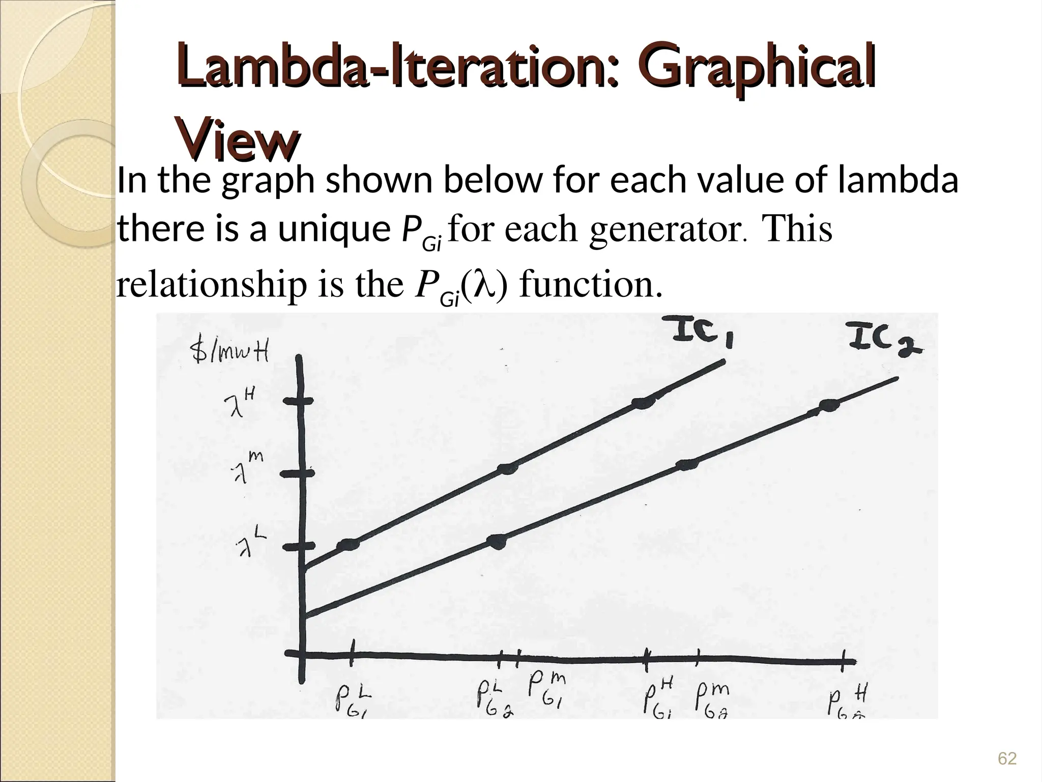
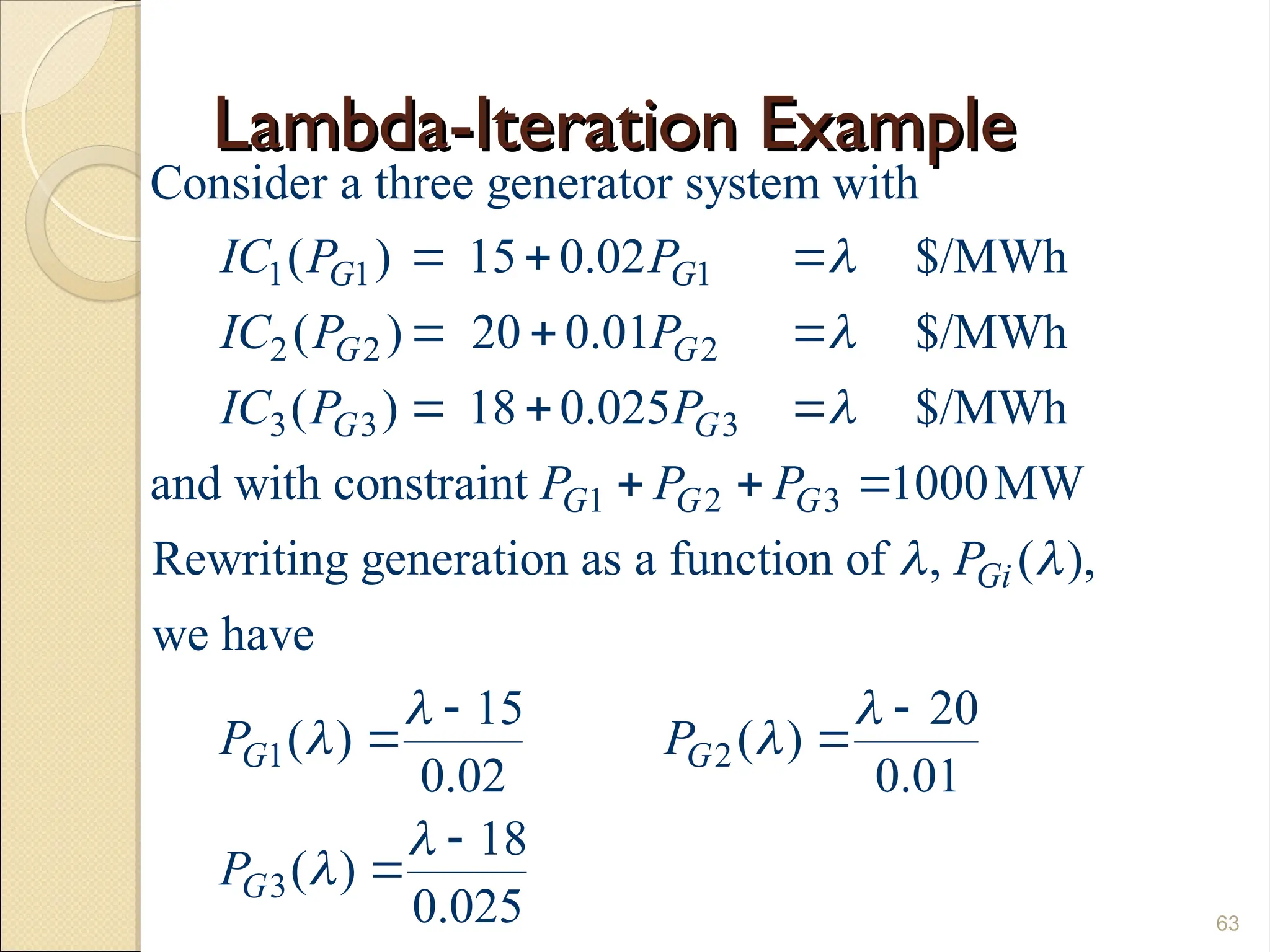
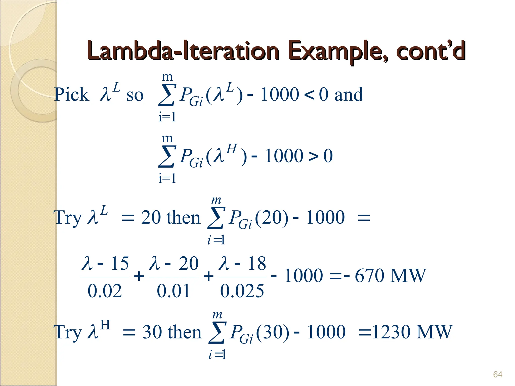
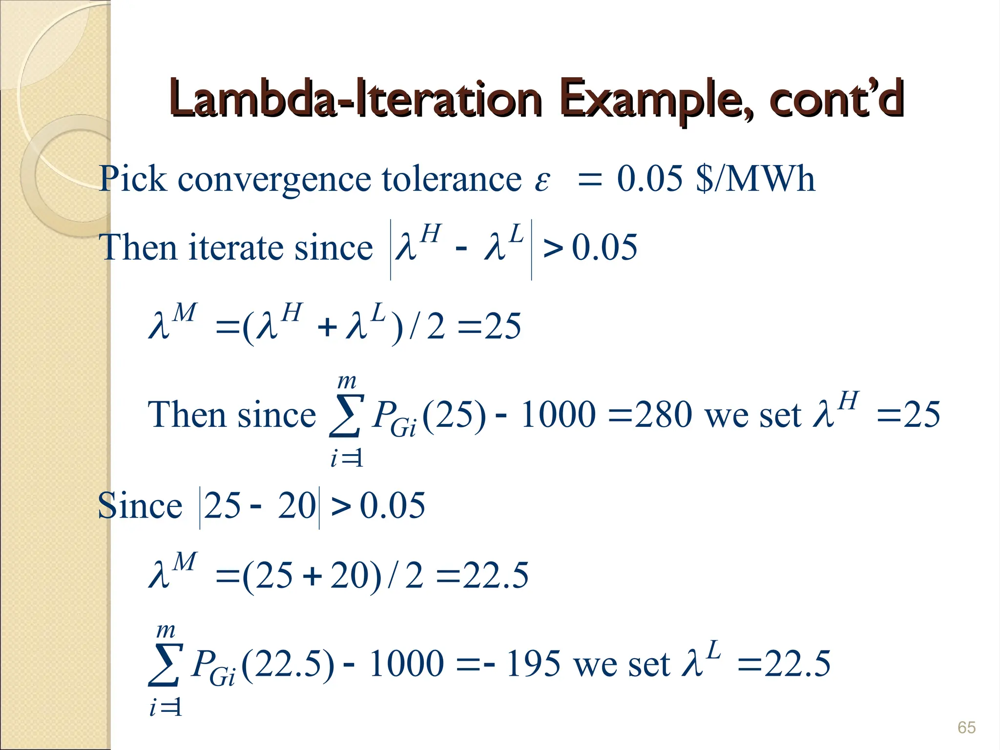
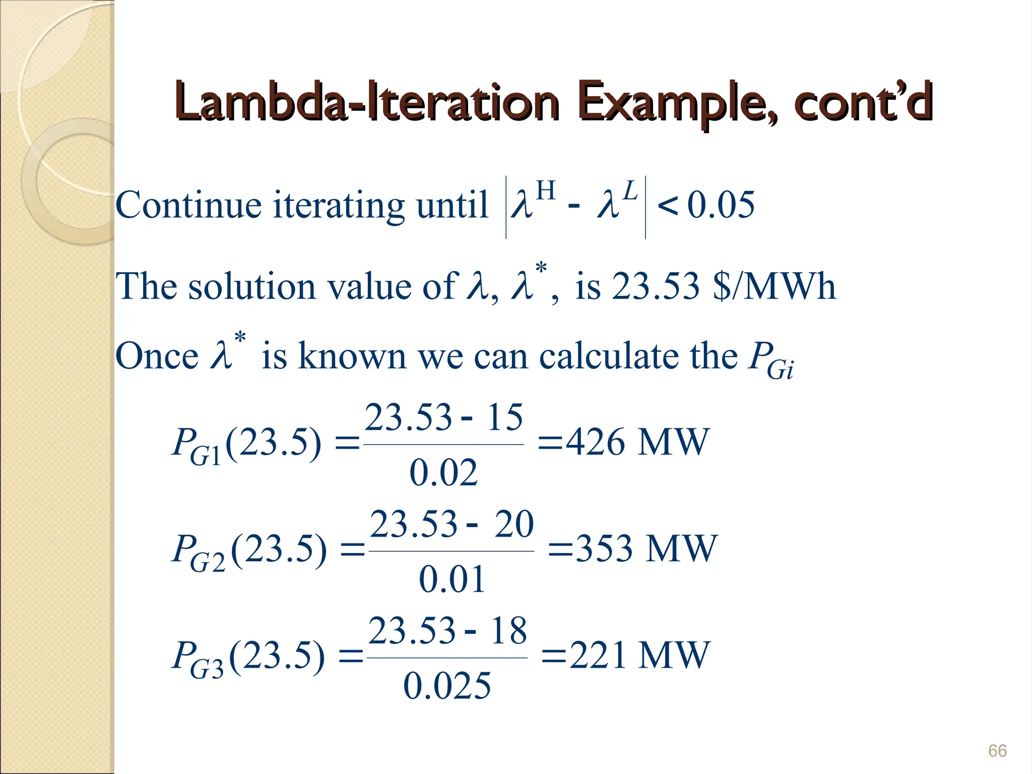
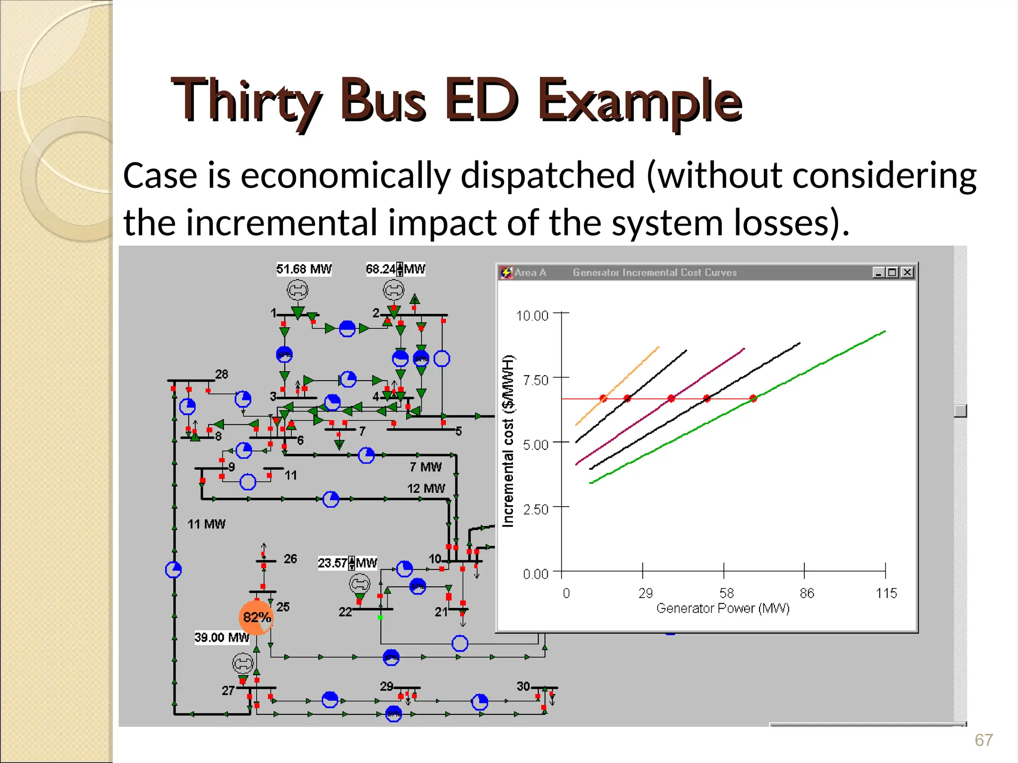
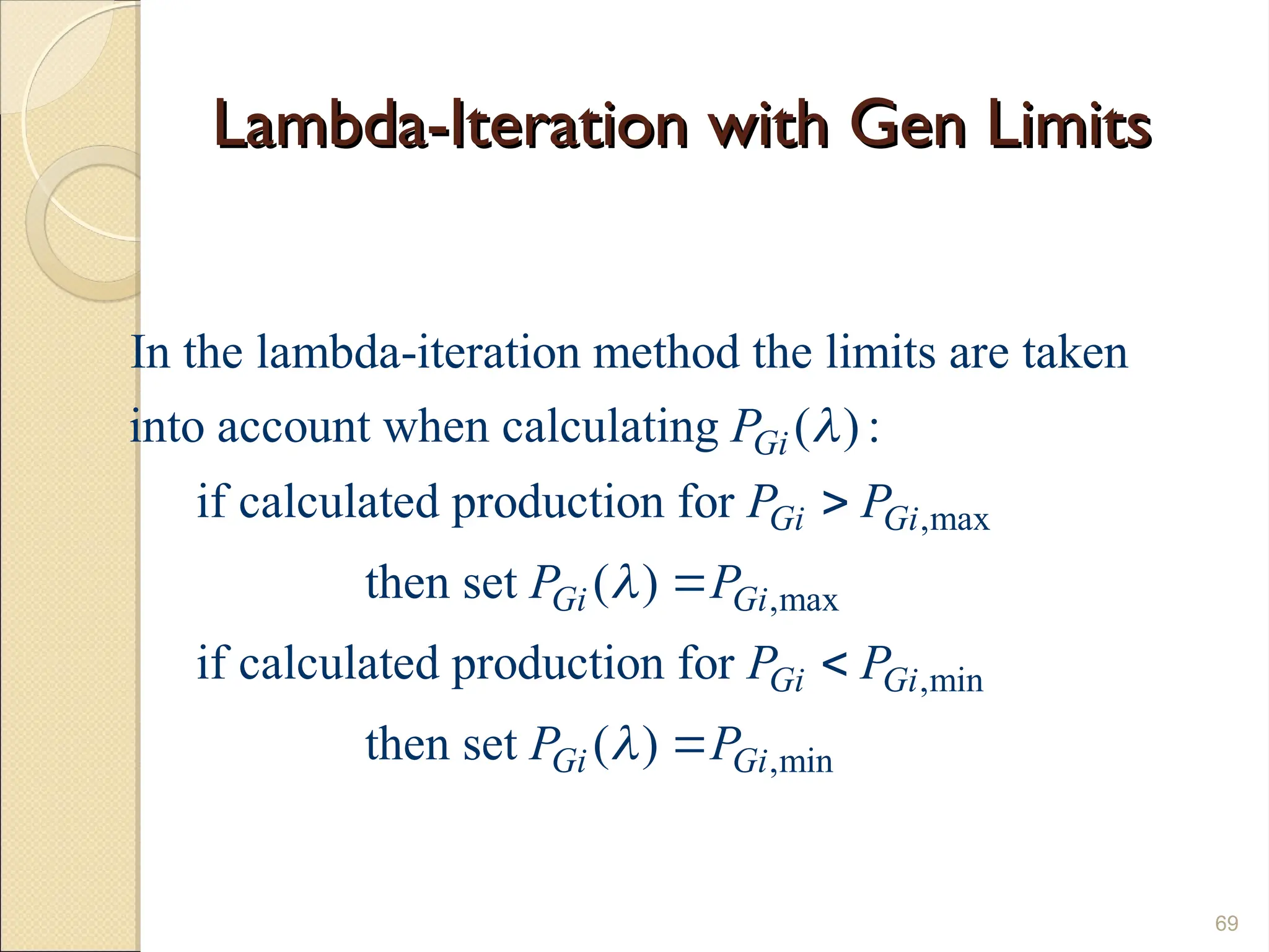
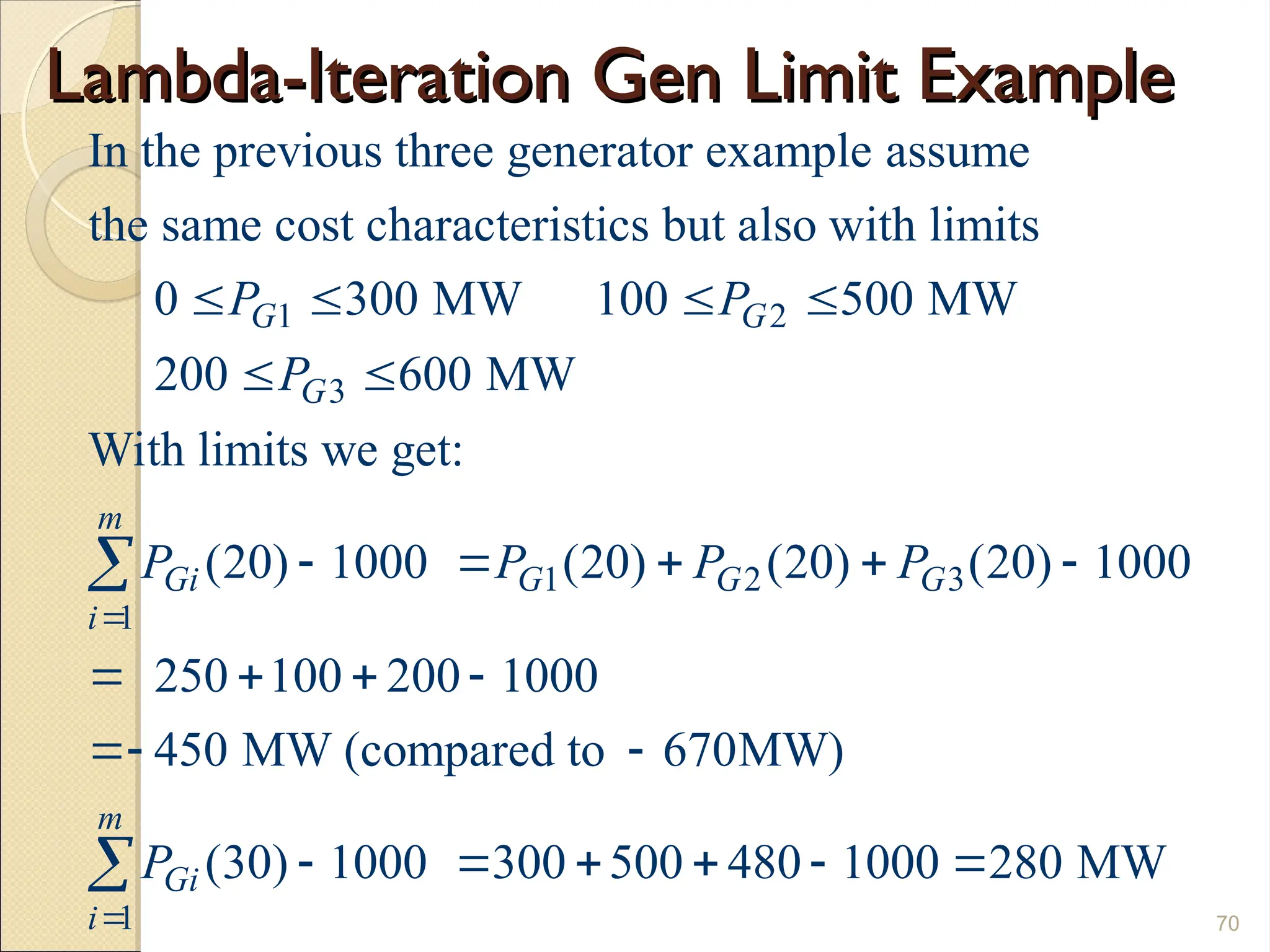
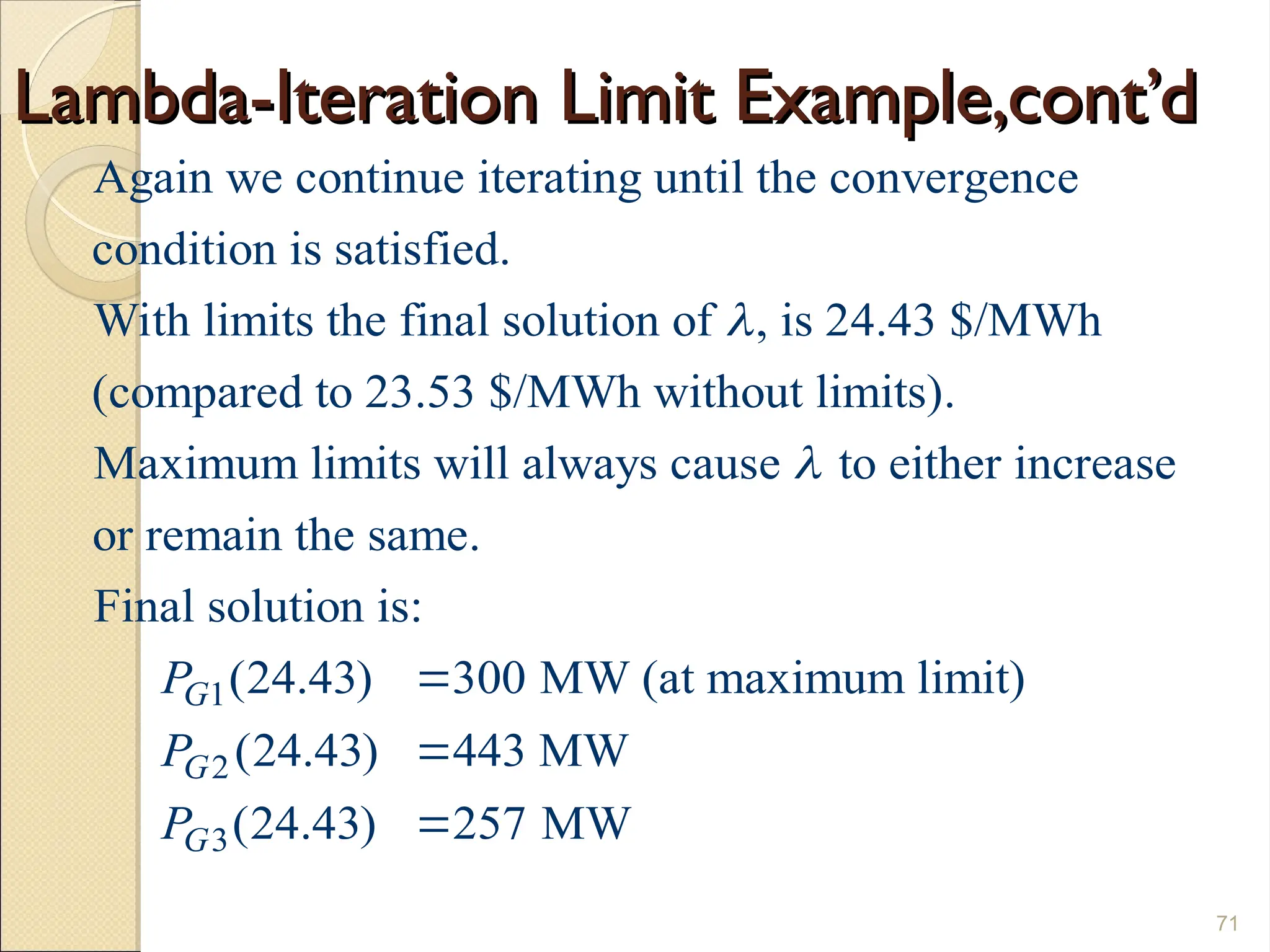
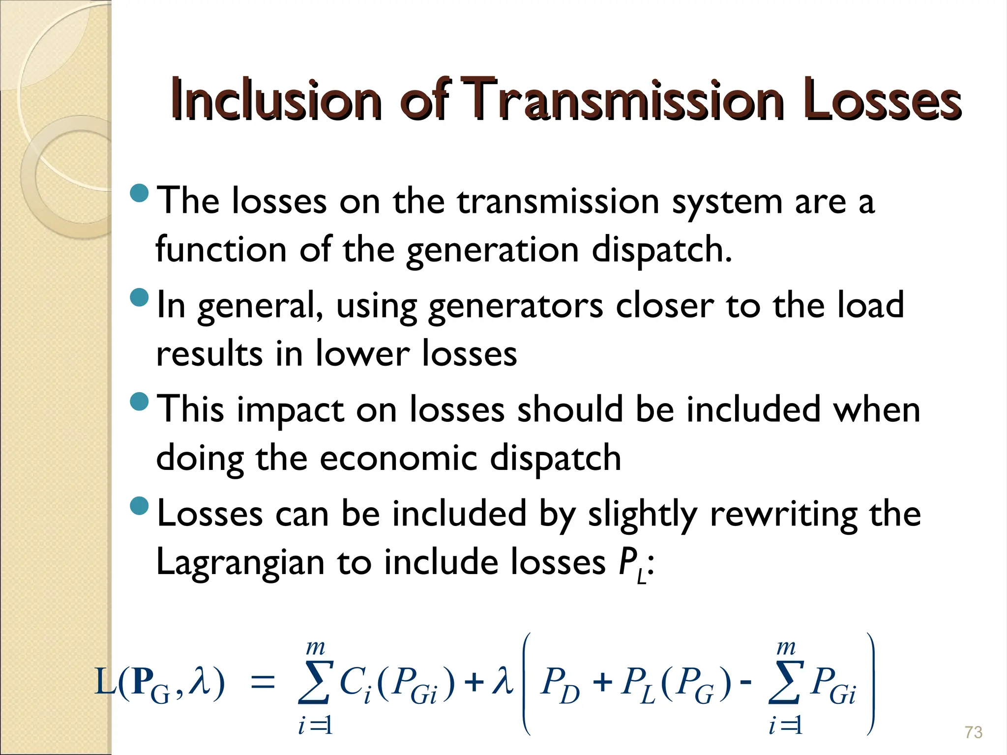
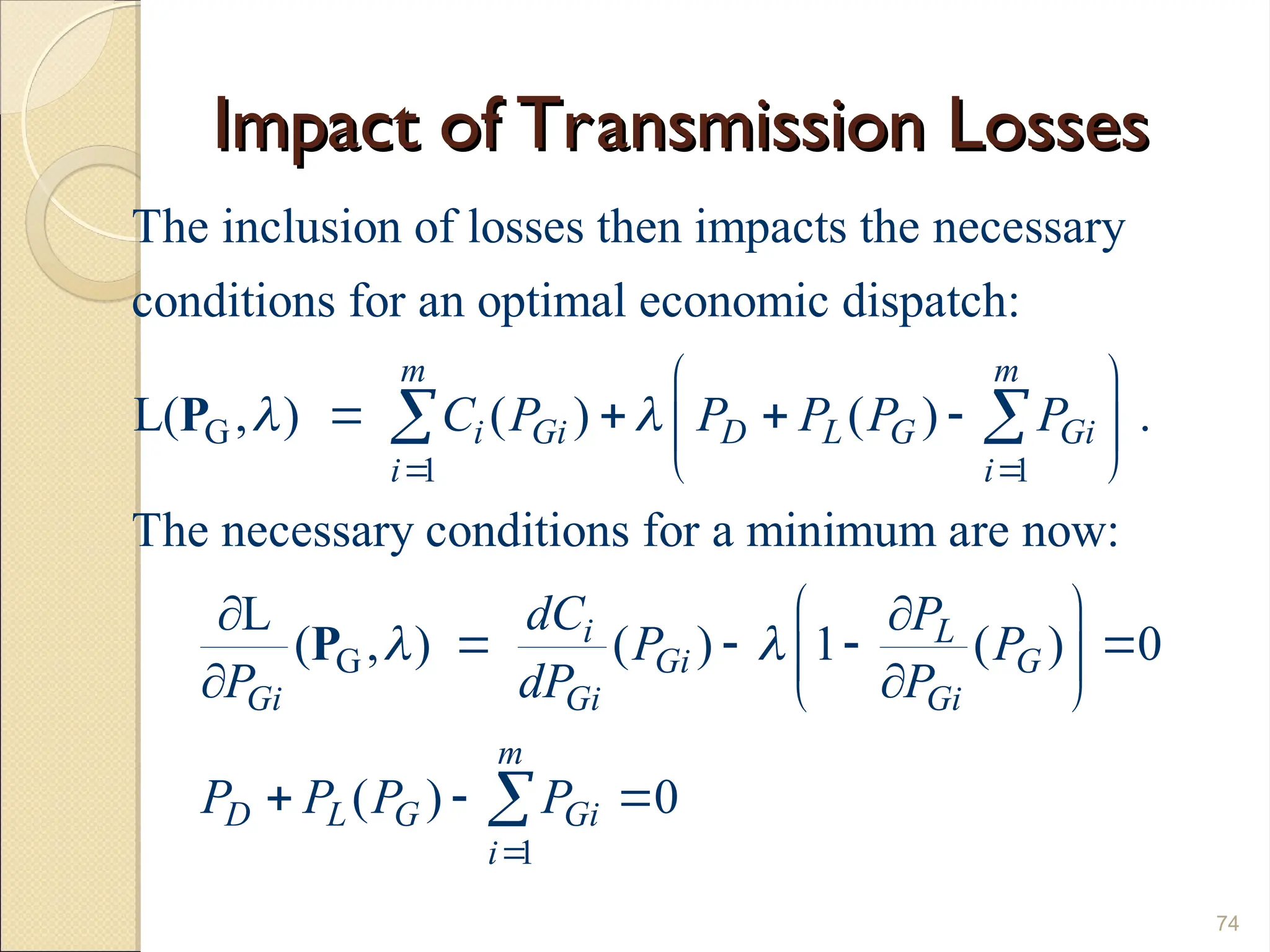
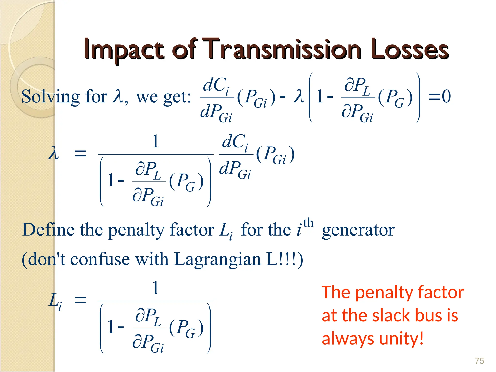
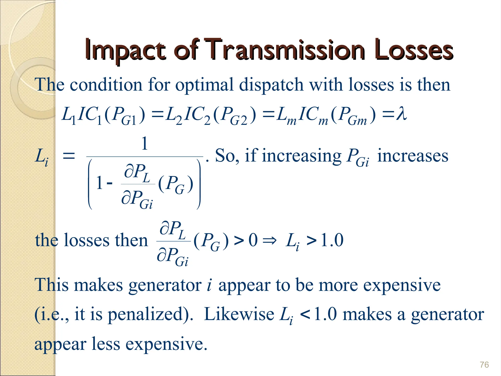
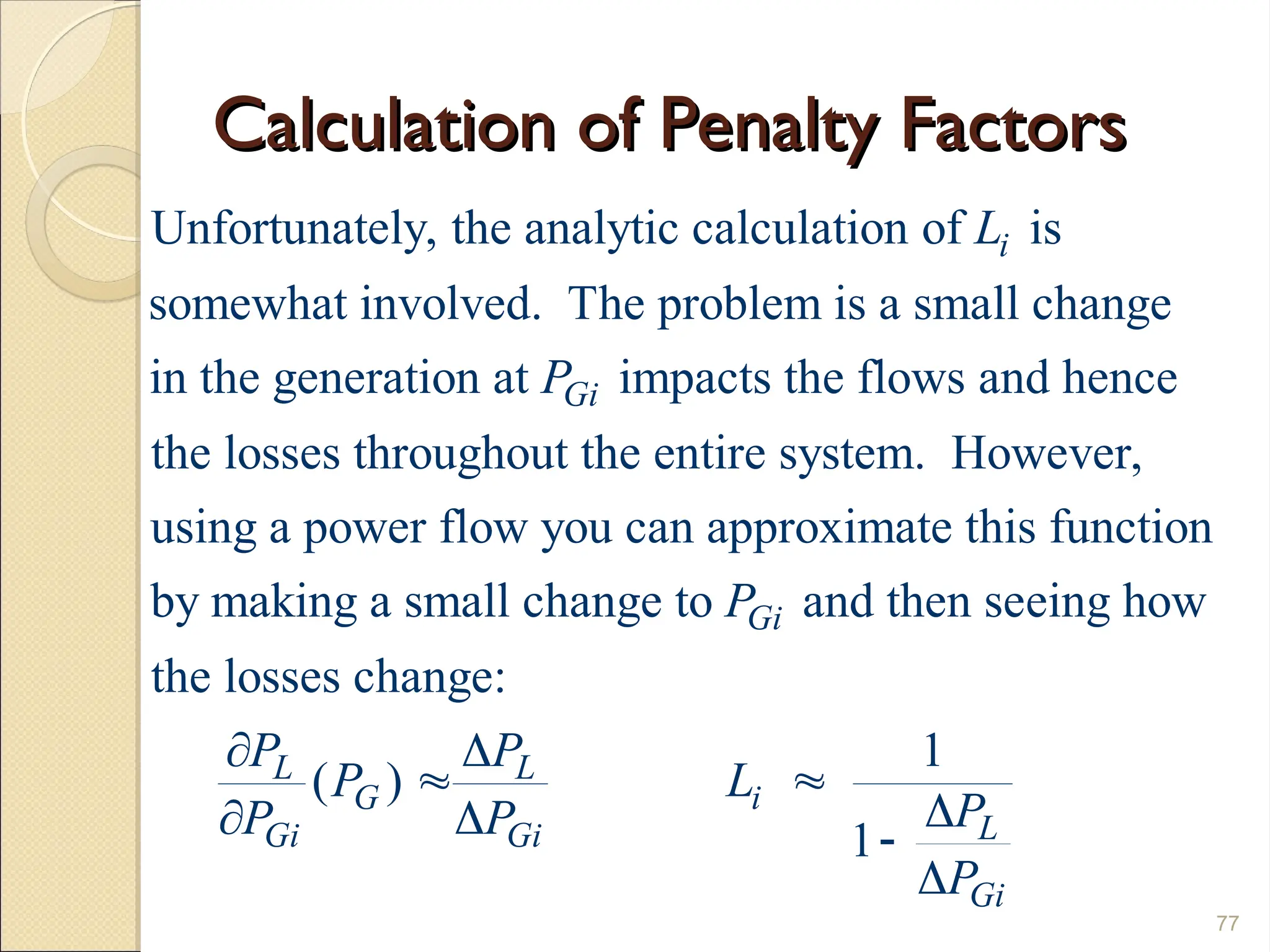
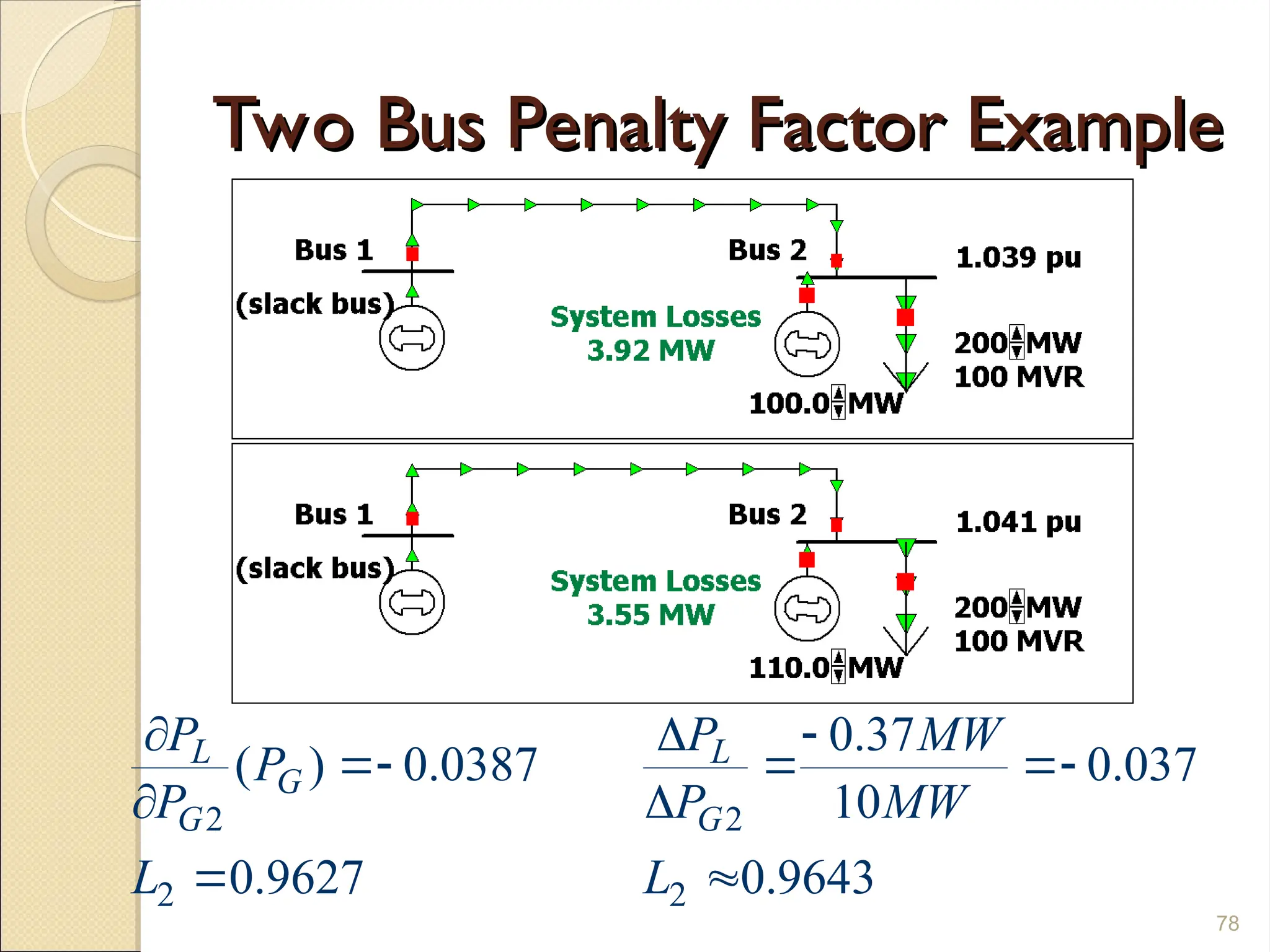
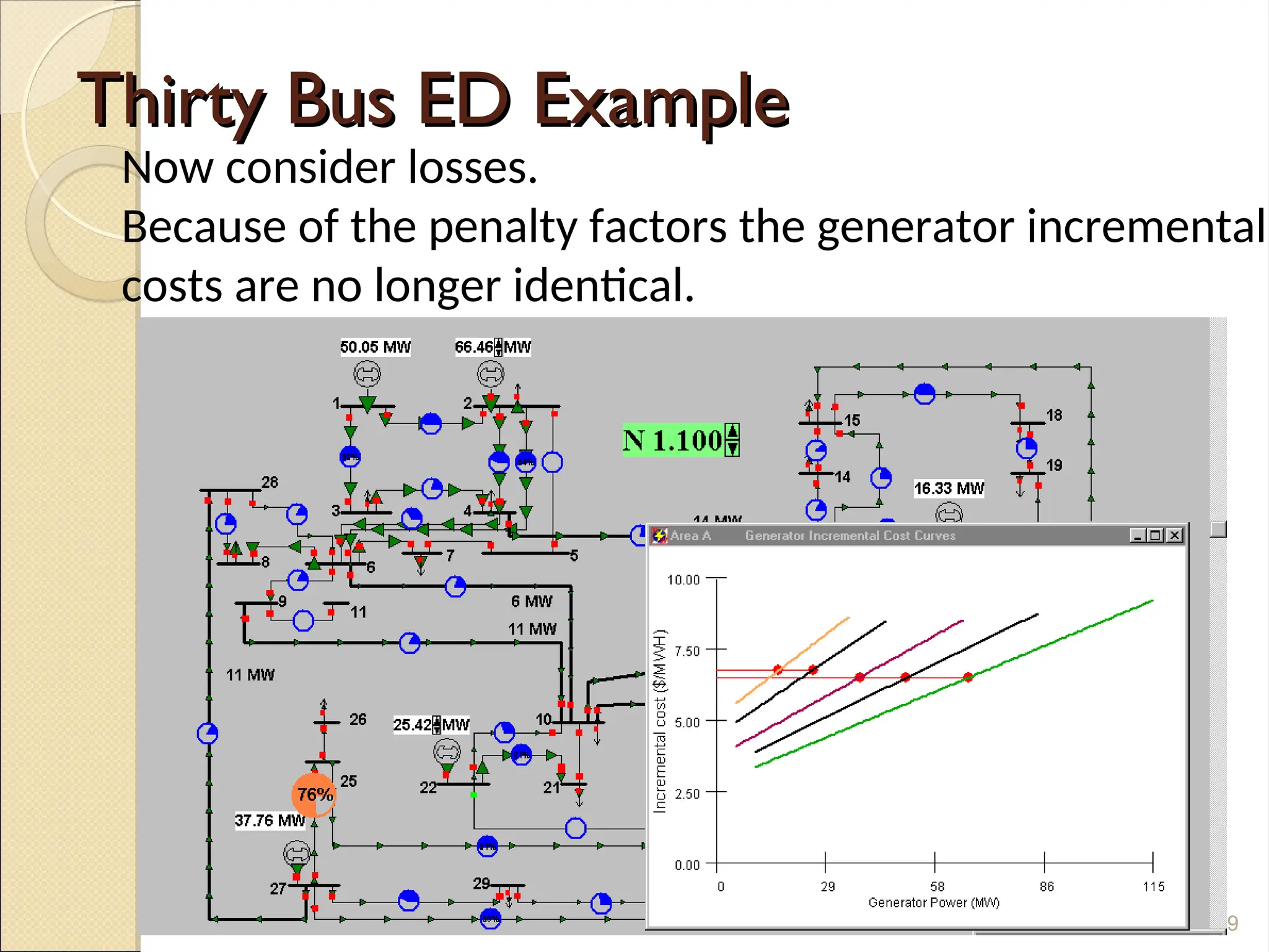
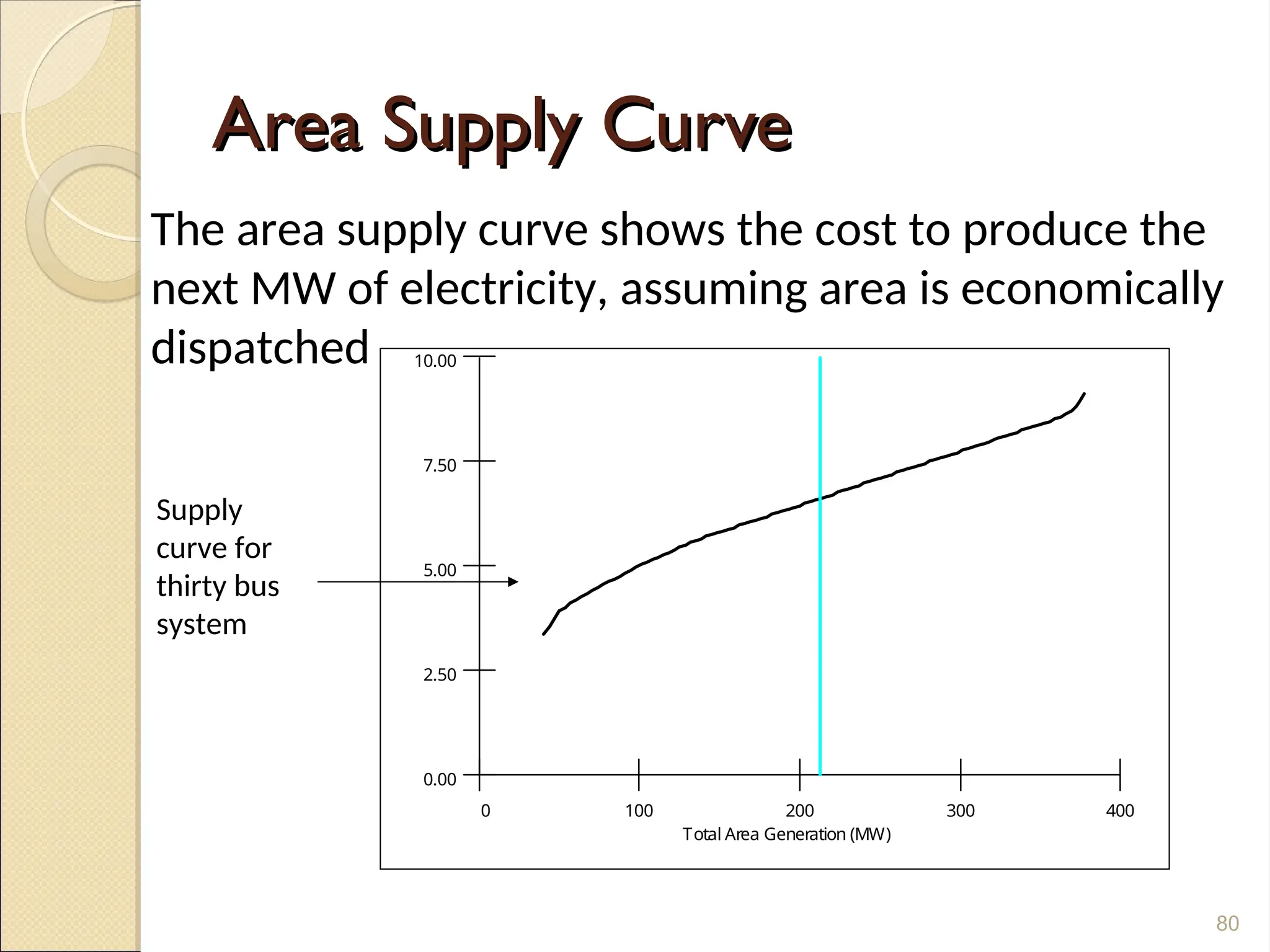
1
UNIT-IV
UNIT COMMITMENT AND
ECONOMIC DISPATCH
2
Syllabus:
Statement of unit commitment problem-
constraints: spinning reserve, thermal unit
constraints, hydro constraints, fuel constraints
and other constraints. Solution methods: priority
list methods, forward dynamic programming
approach. Numerical problems only in priority
list method using full load average production
cost. Statement of economic dispatch problem-
cost of generation-incremental cost curve –co-
ordination equations without loss and with loss-
solution by direct method and lamda iteration
method(No derivation of loss coefficients)
3
Thermal unit constraints
 A thermal unit can with stand only graded
temperature charges and is required to
take some hours to bring the unit on-line.
 For thermal plants, one hour is the
smallest time period that should be
considered for unit commitment solution
as the start-up and shut-down time for
many units is of this order.
4
 Minimum up time
 Once the unit is running, it should not be turned off
immediately
 Minimum down time:
 Once the unit is decommitted, there is a minimum
time before it can be recommitted.
 Crew constraints:
 If a plant consist of two or more units, they cannot
both be turned on at the same time. Since there are
not enough crew members to attend both units
while starting up
5
 Start-up cost:
 It is dependent upon the down-time of
the unit i.e., the time interval between
shut-down and restart.
 Start-up cost when cooling :
 During down time period, the unit’s
boiler to cool down and then heat back
up tp operating temperature in time for a
scheduled turn on
6
Start – up cost when banking
(shut-down cost)
(shut-down cost)
 During shut-down period, the boiler may
be allowed to cool down and thus no
shut down cost will be incurred.
7
Hydro constraints
Hydro constraints
 In hydro-thermal scheduling, to allocate
maximum hydro units during rainy seasons
and to allocate thermal units during
remaining periods.
Fuel constraints:
If thermal and hydro sources are available, a
combined operation is economic and
advantageous i.e., to minimize the fuel cost
of thermal unit over a commitment period.
8
Daily load curve
Daily load curve
9
UNIT COMMITMENT
UNIT COMMITMENT
SOLUTION METHODS
SOLUTION METHODS
 To form loading pattern for M – Periods
using load curve.
 • Commit possible number of units to be
operated to meet out the load.
 • To determine the load dispatch for all
feasible combination of solution for each
load level and satisfying operating limits of
each units.
10
Brute Force Technique or
Simple Priority List scheme
11
Peak – Valley” pattern
12
If the operation of the system is to be optimized, units must be shut down as
the load gets down and then recommitted as it goes back up
Priority List method (Using full load average production cost
FLAPC
FLAPC
 Determine the full load average produce production cast for each units.
 From priority order based on average production cost, (ascending order)
 Commit number of units corresponding, to the priority order.
 Calculate from economic dispatch problem for the feasible combinations only.
 For load curve, each hour load is verifying. Assume load is dropping or decreasing,
determine whether dropping or decreasing, determine whether dropping the next unit will
supply generation and spinning reserve. If not continue as it is, if yes, go to next step.
 Determine the number of hours, H, before the unit will be needed again.
 Check H < Minimum shunt down time
 If yes, go to last step
 If not, go to next step
 Calculate two costs
 Sum of hourly production cost for the next H hours with the unit up.
 Recalculate the same for the unit down + start-up cost for either cooling or banking.
 If the second case is less expensive, the unit should be on.
 Repeat this procedure until the priority list
13
Dynamic Programming Method
14
STATEMENT OF ECONOMIC
DISPATCH PROBLEM
DISPATCH PROBLEM
15
Necessity of economic dispatch
 In many cases economic factor and the availability of priority essentials
such as coal, water etc. dictate that new generating plants is located at
greater distances from the load centers.
 The installation of larger blocks of power has resulted in the necessity of
transmitting power out of a given area until the load in that area is equal to
the new block of installed capacity.
 Power systems are inter connecting for purposes of economy interchange
and reduction of reserve capacity.
 In a number of areas of the country, the cost of fuel is rapidly increasing
16
Generation Strategy
Generation Strategy
17
Daily load curve
Daily load curve
 Base load units
 Intermediate units
 Peaking units
 Reserve units
18
Base load units
Base load units
 Nuclear units full under this category. It is
necessary to maintain the thermal balance
of the nuclear reactor and steam system.
Hence it is desirable to maintain the
megawatt output of such units at a
constants level.
19
Intermediate units
Intermediate units
 Hydro powered units are best suited in
cases where the power output has to be
regulated. The output is controlled by
changing the water flow through the
turbine. In the absence of hydro power
thermal units has to be used
20
Peaking
Peaking units
units
 In case of sudden increase in the load the
best choice is the gas – tubing driving
generators pumped hydro storage and
compressed gas are the special type of
peaking equipment which can be used for
this purpose
21
Reserve units:
Reserve units:
Generators which are maintained at partial output and generators which are
ready for operation comes under this category
Problems involved:
 Hourly shifting of the power demand
 Generating unit must be regularly
maintained and, in case of nuclear units, it
must be refueled.
 Ability of the system to match the
generation to the load not only over the 24
hours daily time span but over seasons
and years
22
Economic Dispatch
Economic Dispatch
 The purpose of economic dispatch or
optimal dispatch is to reduce fuel cost for
the power system. By economic load
scheduling, we mean to find the
generation of the different generations of
plants, so that the total fuel cost is
minimum and at the same time the total
demand and losses at any instant must be
met by the total generation
23
Methods
Methods
 Base load method: where the most
efficient unit is loaded to its maximum
capability, then the second most efficient
unit is loaded etc.
 Best point loading: (Incremental
method) where units are successively
loaded to their lowest heat rate point
beginning with the most efficient unit and
working down to the least efficient unit.
24
OPTIMAL OPERATION OF
GENERATORS ON A BUSBAR
 Generator Operating Cost :
 The total generator operating cost
includes fuel cost, cost of transmission
loss, labour and maintenance cost. For
simplicity, fuel, cost is considered to be
variable
25
Cost of generation depends on
operating constraints or system
constraints
constraints
 Equality constraint
 Inequality constraints
 Voltage constraints
 Running space capacity constraints
 Transformer tap settings
 Transmission line constraints
 Network securing
26
Equality constraint
Equality constraint
27
Inequality constraints
28
Voltage constraints
Voltage constraints
29
Running and Transformer tap
30
Transmission line constraints and
Network securing
Network securing
31
Input – output characteristics
of a generating unit
32
HEAT RATE CURVE
HEAT RATE CURVE
33
34
Incremental heat rate
Cost function
Cost function
35
Incremental Cost Curve of Received Power (or)
System Incremental Cost (or) Incremental Fuel
Cost (IC) (or) Incremental Operating cost
36
Incremental fuel cost curve
37
Incremental cost curve for
thermal power plant
thermal power plant
38
Input- output curve and incremental
cost curve for hydro power plant
39
Two Area System
Two Area System
40
Three possible cases are:
1. Area A is generating power at a lower incremental cost than area B and
possesses extra spinning reserve.
2. Area B will save money simply by purchasing extra MW from area A
which is generating power at a lower cost than area B.
3. Area A would benefit economically from selling power to area B as long
as area B is willing to pay a price.
Economic Dispatch: Formulation
The goal of economic dispatch is to determine
the generation dispatch that minimizes the
instantaneous operating cost, subject to the
constraint that total generation = total load +
losses
41
T
1
1
Minimize C ( )
Such that
m
i Gi
i
m
Gi D Losses
i
C P
P P P


 



Initially we'll
ignore generator
limits and the
losses
Unconstrained Minimization
This is a minimization problem with a single equality
constraint
For an unconstrained minimization a necessary (but not
sufficient) condition for a minimum is the gradient of the
function must be zero,
The gradient generalizes the first derivative for multi-
variable problems:
42
1 2
( ) ( ) ( )
( ) , , ,
n
x x x
 
  
  
  
 
f x f x f x
f x 

( )
 
f x 0
Minimization with Equality Constraint
When the minimization is constrained with an
equality constraint we can solve the problem using
the method of Lagrange Multipliers
Key idea is to represent a constrained minimization
problem as an unconstrained problem.
43
That is, for the general problem
minimize ( ) s.t. ( )
We define the Lagrangian L( , ) ( ) ( )
Then a necessary condition for a minimum is the
L ( , ) 0 and L ( , ) 0
T

 
   
x λ
f x g x 0
x λ f x λ g x
x λ x λ
Economic Dispatch Lagrangian
44
G
1 1
G
For the economic dispatch we have a minimization
constrained with a single equality constraint
L( , ) ( ) ( ) (no losses)
The necessary conditions for a minimum are
L
( , )
m m
i Gi D Gi
i i
Gi
C P P P
dC
P
 

 
  



 
P
P
1
( ) 0 (for 1 to )
0
i
Gi
Gi
m
D Gi
i
P i m
dP
P P


  
 

Economic Dispatch Example
45
1 2
2
1 1 1 1
2
2 2 2 2
1
1
1
What is economic dispatch for a two generator
system 500 MW and
( ) 1000 20 0.01 $/h
( ) 400 15 0.03 $/h
Using the Lagrange multiplier method we know:
( ) 20 0.0
D G G
G G G
G G G
G
G
P P P
C P P P
C P P P
dC
P
dP

  
  
  
   1
2
2 2
2
1 2
2 0
( ) 15 0.06 0
500 0
G
G G
G
G G
P
dC
P P
dP
P P

 
 
    
  
Economic Dispatch Example, cont’d
46
1
2
1 2
1
2
1
2
We therefore need to solve three linear equations
20 0.02 0
15 0.06 0
500 0
0.02 0 1 20
0 0.06 1 15
1 1 0 500
312.5 MW
187.5 MW
26.2 $/MW
G
G
G G
G
G
G
G
P
P
P P
P
P
P
P




  
  
  
 
     
     
  
     
  
     
     
 
  
 
 
  h
 
 
 
 
 
Inequality constraints
47
Coordination Equation without
loss
loss
48
Cont/.,
Cont/.,
49
Con/.,
Con/.,
50
Coordination equation with Loss or
exact equation
exact equation
51
Contin/.,
Contin/.,
52
Optimum Allocated of Generator (Bij)
Coefficient are considered
53
Contin/.,
Contin/.,
54
Contin/.,
Contin/.,
55
Contin/.,
Contin/.,
56
57
Economic dispatch example, cont’d
 At the solution, both generators have the same marginal
(or incremental) cost, and this common marginal cost is
equal to λ.
 Intuition behind solution:
◦ If marginal costs of generators were different, then by
decreasing production at higher marginal cost generator, and
increasing production at lower marginal cost generator we
could lower overall costs.
◦ Generalizes to any number of generators.
 If demand changes, then change in total costs can be
estimated from λ.
58
Economic dispatch example, cont’d
 Another way to solve the equations is to:
◦ Rearrange the first two equations to solve for PG1
and PG2 in terms of λ,
◦ Plug into third equation and solve for λ,
◦ Use the solved value of λ to evaluate PG1 and PG2.
 This works even when relationship between
generation levels and λ is more complicated:
◦ Equations are more complicated than linear when
there are maximum and minimum generation
limits or we consider losses.
59
Lambda-Iteration Solution Method
 Discussion on previous page leads to “lambda-
iteration” method:
◦ this method requires a unique mapping from a value of
lambda (marginal cost) to each generator’s MW output:
◦ for any choice of lambda (common marginal cost), the
generators collectively produce a total MW output,
◦ the method then starts with values of lambda below and
above the optimal value (corresponding to too little and
too much total output), and then iteratively brackets the
optimal value.
•
6
( ).
Gi
P 
Lambda-Iteration Algorithm
61
L H
1 1
H L
M H L
H M
1
L M
Pick and such that
( ) 0 ( ) 0
While Do
( )/2
If ( ) 0 Then
Else
End While
m m
L H
Gi D Gi D
i i
m
M
Gi D
i
P P P P
P P
 
 
  
  
  
 
 

   
 
 
  

 

Lambda-Iteration: Graphical
View
View
62
In the graph shown below for each value of lambda
there is a unique PGi for each generator. This
relationship is the PGi() function.
Lambda-Iteration Example
63
1 1 1
2 2 2
3 3 3
1 2 3
Consider a three generator system with
( ) 15 0.02 $/MWh
( ) 20 0.01 $/MWh
( ) 18 0.025 $/MWh
and with constraint 1000MW
Rewriting generation as a function of , (
G G
G G
G G
G G G
Gi
IC P P
IC P P
IC P P
P P P
P




  
  
  
  
1 2
3
),
we have
15 20
( ) ( )
0.02 0.01
18
( )
0.025
G G
G
P P
P

 
 


 
 


Lambda-Iteration Example, cont’d
64
m
i=1
m
i=1
1
H
1
Pick so ( ) 1000 0 and
( ) 1000 0
Try 20 then (20) 1000
15 20 18
1000 670 MW
0.02 0.01 0.025
Try 30 then (30) 1000 1230 MW
L L
Gi
H
Gi
m
L
Gi
i
m
Gi
i
P
P
P
P
 


  



 
 
  
  
   
  




Lambda-Iteration Example, cont’d
65
1
1
Pick convergence tolerance 0.05 $/MWh
Then iterate since 0.05
( )/ 2 25
Then since (25) 1000 280 we set 25
Since 25 20 0.05
(25 20)/ 2 22.5
(22.5) 1000 195 we set 2
H L
M H L
m
H
Gi
i
M
m
L
Gi
i
P
P

 
  






 
  
  
 
  
  

 2.5
Lambda-Iteration Example, cont’d
66
H
*
*
1
2
3
Continue iterating until 0.05
The solution value of , , is 23.53 $/MWh
Once is known we can calculate the
23.53 15
(23.5) 426 MW
0.02
23.53 20
(23.5) 353 MW
0.01
23.53 18
(23.5)
0.025
L
Gi
G
G
G
P
P
P
P
 
 

 

 

 

 221 MW

Thirty Bus ED Example
67
Case is economically dispatched (without considering
the incremental impact of the system losses).
Generator MW Limits
Generator MW Limits
Generators have limits on the minimum and
maximum amount of power they can
produce
Typically the minimum limit is not zero.
Because of varying system economics usually
many generators in a system are operated at
their maximum MW limits:
Baseload generators are at their maximum limits
except during the off-peak.
68
Lambda-Iteration with Gen Limits
69
,max
,max
In the lambda-iteration method the limits are taken
into account when calculating ( ) :
if calculated production for
then set ( )
if calculated production for
Gi
Gi Gi
Gi Gi
P
P P
P P




,min
,min
then set ( )
Gi Gi
Gi Gi
P P
P P



Lambda-Iteration Gen Limit Example
70
1 2
3
1 2 3
1
In the previous three generator example assume
the same cost characteristics but also with limits
0 300 MW 100 500 MW
200 600 MW
With limits we get:
(20) 1000 (20) (20) (20) 10
G G
G
m
Gi G G G
i
P P
P
P P P P

   
 
    

1
00
250 100 200 1000
450 MW (compared to 670MW)
(30) 1000 300 500 480 1000 280 MW
m
Gi
i
P

   
 
     

Lambda-Iteration Limit Example,cont’d
71
Again we continue iterating until the convergence
condition is satisfied.
With limits the final solution of , is 24.43 $/MWh
(compared to 23.53 $/MWh without limits).
Maximum limits will always caus

1
2
3
e to either increase
or remain the same.
Final solution is:
(24.43) 300 MW (at maximum limit)
(24.43) 443 MW
(24.43) 257 MW
G
G
G
P
P
P




Back of Envelope Values
$/MWhr = fuelcost * heatrate + variable O&M
Typical incremental costs can be roughly
approximated:
– Typical heatrate for a coal plant is 10, modern
combustion turbine is 10, combined cycle plant is 6 to 8,
older combustion turbine 15.
– Fuel costs ($/MBtu) are quite variable, with current
values around 2 for coal, 3 to 5 for natural gas, 0.5 for
nuclear, probably 10 for fuel oil.
– Hydro costs tend to be quite low, but are fuel (water)
constrained
– Wind and solar costs are zero.
72
Inclusion of Transmission Losses
The losses on the transmission system are a
function of the generation dispatch.
In general, using generators closer to the load
results in lower losses
This impact on losses should be included when
doing the economic dispatch
Losses can be included by slightly rewriting the
Lagrangian to include losses PL:
73
G
1 1
L( , ) ( ) ( )
m m
i Gi D L G Gi
i i
C P P P P P
 
 
 
   
 
 
 
P
Impact of Transmission Losses
74
G
1 1
G
The inclusion of losses then impacts the necessary
conditions for an optimal economic dispatch:
L( , ) ( ) ( ) .
The necessary conditions for a minimum are now:
L
(
m m
i Gi D L G Gi
i i
Gi
C P P P P P
P
 
 
 
   
 
 


 
P
P
1
, ) ( ) 1 ( ) 0
( ) 0
i L
Gi G
Gi Gi
m
D L G Gi
i
dC P
P P
dP P
P P P P
 

 

   
 

 
  

Impact of Transmission Losses
75
th
Solving for , we get: ( ) 1 ( ) 0
1
( )
1 ( )
Define the penalty factor for the generator
(don't confuse with Lagrangian L!!!)
1
1 ( )
i L
Gi G
Gi Gi
i
Gi
Gi
L
G
Gi
i
i
L
G
Gi
dC P
P P
dP P
dC
P
dP
P
P
P
L i
L
P
P
P
 

 

  
 

 

 


 

 

 

 




The penalty factor
at the slack bus is
always unity!
Impact of Transmission Losses
76
1 1 1 2 2 2
The condition for optimal dispatch with losses is then
( ) ( ) ( )
1
. So, if increasing increases
1 ( )
the losses then ( ) 0 1.0
This makes generator
G G m m Gm
i Gi
L
G
Gi
L
G i
Gi
L IC P L IC P L IC P
L P
P
P
P
P
P L
P

  

 


 

 

  

appear to be more expensive
(i.e., it is penalized). Likewise 1.0 makes a generator
appear less expensive.
i
i
L 
Calculation of Penalty Factors
77
Unfortunately, the analytic calculation of is
somewhat involved. The problem is a small change
in the generation at impacts the flows and hence
the losses throughout the entire system. However,
i
Gi
L
P
using a power flow you can approximate this function
by making a small change to and then seeing how
the losses change:
1
( )
1
Gi
L L
G i
L
Gi Gi
Gi
P
P P
P L
P
P P
P
 
 

  

Two Bus Penalty Factor Example
78
2 2
2 2
0.37
( ) 0.0387 0.037
10
0.9627 0.9643
L L
G
G G
P P MW
P
P P MW
L L
  
  
 
 
Thirty Bus ED Example
79
Now consider losses.
Because of the penalty factors the generator incremental
costs are no longer identical.
Area Supply Curve
Area Supply Curve
80
0 100 200 300 400
Total Area Generation (MW)
0.00
2.50
5.00
7.50
10.00
The area supply curve shows the cost to produce the
next MW of electricity, assuming area is economically
dispatched
Supply
curve for
thirty bus
system
Economic Dispatch - Summary
Economic dispatch determines the best way to
minimize the current generator operating costs.
The lambda-iteration method is a good approach
for solving the economic dispatch problem:
– generator limits are easily handled,
– penalty factors are used to consider the impact of
losses.
Economic dispatch is not concerned with
determining which units to turn on/off (this is the
unit commitment problem).
Basic form of economic dispatch ignores the
transmission system limitations.
81
Security Constrained ED
or Optimal Power Flow
Transmission constraints often limit ability to
use lower cost power.
Such limits require deviations from what would
otherwise be minimum cost dispatch in order to
maintain system “security.”
Need to solve or approximate power flow in
order to consider transmission constraints.
82
Security Constrained ED
or Optimal Power Flow
The goal of a security constrained ED or optimal
power flow (OPF) is to determine the “best”
way to instantaneously operate a power system,
considering transmission limits.
Usually “best” = minimizing operating cost, while
keeping flows on transmission below limits.
In three bus case the generation at bus 3 must
be limited to avoid overloading the line from bus
3 to bus 2.
83
Security Constrained Dispatch
Bus 2 Bus 1
Bus 3
Home Area
Scheduled Transactions
357 MW
179 MVR
194 MW
448 MW
19 MVR
232 MVR
179 MW
89 MVR
1.00 PU
-22 MW
4 MVR
22 MW
-4 MVR
-142 MW
49 MVR
145 MW
-37 MVR
124 MW
-33 MVR
-122 MW
41 MVR
1.00 PU
1.00 PU
0 MW
37 MVR
100%
100%
100 MW
OFF AGC
AVR ON
AGC ON
AVR ON
100.0 MW
84
Need to dispatch to keep line
from bus 3 to bus 2 from overloading
Multi-Area Operation
In multi-area system, “rules” have been established
regarding transactions on tie-lines:
– In Eastern interconnection, in principle, up to “nominal”
thermal interconnection capacity,
– In Western interconnection there are more complicated
rules
The actual power that flows through the entire
network depends on the impedance of the transmission
lines, and ultimately determine what are acceptable
patterns of dispatch:
Can result in need to “curtail” transactions that otherwise
satisfy rules.
Economically uncompensated flow through other areas
is known as “parallel path” or “loop flows.”
Since ERCOT is one area, all of the flows on AC lines
are inside ERCOT and there is no uncompensated flow
on AC lines.
85
Seven Bus Case: One-line
Top Area Cost
Left Area Cost Right Area Cost
1
2
3 4
5
6 7
106 MW
168 MW
200 MW 201 MW
110 MW
40 MVR
80 MW
30 MVR
130 MW
40 MVR
40 MW
20 MVR
1.00 PU
1.01 PU
1.04 PU
1.04 PU
1.04 PU
0.99 PU
1.05 PU
62 MW
-61 MW
44 MW -42 MW -31 MW 31 MW
38 MW
-37 MW
79 MW -77 MW
-32 MW
32 MW
-14 MW
-39 MW
40 MW
-20 MW
20 MW
40 MW
-40 MW
94 MW
200 MW
0 MVR
200 MW
0 MVR
20 MW -20 MW
AGC ON
AGC ON
AGC ON
AGC ON
AGC ON
8029 $/MWH
4715 $/MWH
4189 $/MWH
Case Hourly Cost
16933 $/MWH
86
System has
three areas
Left area
has one
bus
Right area has one
bus
Top area
has five
buses
No net
interchange
between
Any areas.
Seven Bus Case: Area View
Area Losses
Area Losses Area Losses
Top
Left Right
-40.1 MW
0.0 MW
0.0 MW
0.0 MW
40.1 MW
40.1 MW
7.09 MW
0.33 MW 0.65 MW
87
System has
40 MW of
“Loop Flow”
Actual
flow
between
areas
Loop flow can result in higher losses
Scheduled
flow
Seven Bus - Loop Flow?
Area Losses
Area Losses Area Losses
Top
Left Right
-4.8 MW
0.0 MW
100.0 MW
0.0 MW
104.8 MW
4.8 MW
9.44 MW
-0.00 MW 4.34 MW
88
100 MW Transaction
between Left and Right
Transaction has
actually decreased
the loop flow
Note that
Top’s
Losses have
increased
from
7.09MW to
9.44 MW

UNIT-4-PPT UNIT COMMITMENT AND ECONOMIC DISPATCH

  • 1.
  • 2.
  • 3.
    Syllabus: Statement of unitcommitment problem- constraints: spinning reserve, thermal unit constraints, hydro constraints, fuel constraints and other constraints. Solution methods: priority list methods, forward dynamic programming approach. Numerical problems only in priority list method using full load average production cost. Statement of economic dispatch problem- cost of generation-incremental cost curve –co- ordination equations without loss and with loss- solution by direct method and lamda iteration method(No derivation of loss coefficients) 3
  • 4.
    Thermal unit constraints Thermalunit constraints  A thermal unit can with stand only graded temperature charges and is required to take some hours to bring the unit on-line.  For thermal plants, one hour is the smallest time period that should be considered for unit commitment solution as the start-up and shut-down time for many units is of this order. 4
  • 5.
     Minimum uptime  Once the unit is running, it should not be turned off immediately  Minimum down time:  Once the unit is decommitted, there is a minimum time before it can be recommitted.  Crew constraints:  If a plant consist of two or more units, they cannot both be turned on at the same time. Since there are not enough crew members to attend both units while starting up 5
  • 6.
     Start-up cost: It is dependent upon the down-time of the unit i.e., the time interval between shut-down and restart.  Start-up cost when cooling :  During down time period, the unit’s boiler to cool down and then heat back up tp operating temperature in time for a scheduled turn on 6
  • 7.
    Start – upcost when banking Start – up cost when banking (shut-down cost) (shut-down cost)  During shut-down period, the boiler may be allowed to cool down and thus no shut down cost will be incurred. 7
  • 8.
    Hydro constraints Hydro constraints In hydro-thermal scheduling, to allocate maximum hydro units during rainy seasons and to allocate thermal units during remaining periods. Fuel constraints: If thermal and hydro sources are available, a combined operation is economic and advantageous i.e., to minimize the fuel cost of thermal unit over a commitment period. 8
  • 9.
  • 10.
    UNIT COMMITMENT UNIT COMMITMENT SOLUTIONMETHODS SOLUTION METHODS  To form loading pattern for M – Periods using load curve.  • Commit possible number of units to be operated to meet out the load.  • To determine the load dispatch for all feasible combination of solution for each load level and satisfying operating limits of each units. 10
  • 11.
    Brute Force Techniqueor Brute Force Technique or Simple Priority List scheme Simple Priority List scheme 11
  • 12.
    Peak – Valley”pattern Peak – Valley” pattern 12 If the operation of the system is to be optimized, units must be shut down as the load gets down and then recommitted as it goes back up
  • 13.
    Priority List method(Using full load average production cost Priority List method (Using full load average production cost FLAPC FLAPC  Determine the full load average produce production cast for each units.  From priority order based on average production cost, (ascending order)  Commit number of units corresponding, to the priority order.  Calculate from economic dispatch problem for the feasible combinations only.  For load curve, each hour load is verifying. Assume load is dropping or decreasing, determine whether dropping or decreasing, determine whether dropping the next unit will supply generation and spinning reserve. If not continue as it is, if yes, go to next step.  Determine the number of hours, H, before the unit will be needed again.  Check H < Minimum shunt down time  If yes, go to last step  If not, go to next step  Calculate two costs  Sum of hourly production cost for the next H hours with the unit up.  Recalculate the same for the unit down + start-up cost for either cooling or banking.  If the second case is less expensive, the unit should be on.  Repeat this procedure until the priority list 13
  • 14.
  • 15.
    STATEMENT OF ECONOMIC STATEMENTOF ECONOMIC DISPATCH PROBLEM DISPATCH PROBLEM 15
  • 16.
    Necessity of economicdispatch Necessity of economic dispatch  In many cases economic factor and the availability of priority essentials such as coal, water etc. dictate that new generating plants is located at greater distances from the load centers.  The installation of larger blocks of power has resulted in the necessity of transmitting power out of a given area until the load in that area is equal to the new block of installed capacity.  Power systems are inter connecting for purposes of economy interchange and reduction of reserve capacity.  In a number of areas of the country, the cost of fuel is rapidly increasing 16
  • 17.
  • 18.
    Daily load curve Dailyload curve  Base load units  Intermediate units  Peaking units  Reserve units 18
  • 19.
    Base load units Baseload units  Nuclear units full under this category. It is necessary to maintain the thermal balance of the nuclear reactor and steam system. Hence it is desirable to maintain the megawatt output of such units at a constants level. 19
  • 20.
    Intermediate units Intermediate units Hydro powered units are best suited in cases where the power output has to be regulated. The output is controlled by changing the water flow through the turbine. In the absence of hydro power thermal units has to be used 20
  • 21.
    Peaking Peaking units units  Incase of sudden increase in the load the best choice is the gas – tubing driving generators pumped hydro storage and compressed gas are the special type of peaking equipment which can be used for this purpose 21
  • 22.
    Reserve units: Reserve units: Generatorswhich are maintained at partial output and generators which are Generators which are maintained at partial output and generators which are ready for operation comes under this category ready for operation comes under this category Problems involved:  Hourly shifting of the power demand  Generating unit must be regularly maintained and, in case of nuclear units, it must be refueled.  Ability of the system to match the generation to the load not only over the 24 hours daily time span but over seasons and years 22
  • 23.
    Economic Dispatch Economic Dispatch The purpose of economic dispatch or optimal dispatch is to reduce fuel cost for the power system. By economic load scheduling, we mean to find the generation of the different generations of plants, so that the total fuel cost is minimum and at the same time the total demand and losses at any instant must be met by the total generation 23
  • 24.
    Methods Methods  Base loadmethod: where the most efficient unit is loaded to its maximum capability, then the second most efficient unit is loaded etc.  Best point loading: (Incremental method) where units are successively loaded to their lowest heat rate point beginning with the most efficient unit and working down to the least efficient unit. 24
  • 25.
    OPTIMAL OPERATION OF OPTIMALOPERATION OF GENERATORS ON A BUSBAR GENERATORS ON A BUSBAR  Generator Operating Cost :  The total generator operating cost includes fuel cost, cost of transmission loss, labour and maintenance cost. For simplicity, fuel, cost is considered to be variable 25
  • 26.
    Cost of generationdepends on Cost of generation depends on operating constraints or system operating constraints or system constraints constraints  Equality constraint  Inequality constraints  Voltage constraints  Running space capacity constraints  Transformer tap settings  Transmission line constraints  Network securing 26
  • 27.
  • 28.
  • 29.
  • 30.
    Running and Transformertap Running and Transformer tap 30
  • 31.
    Transmission line constraintsand Transmission line constraints and Network securing Network securing 31
  • 32.
    Input – outputcharacteristics Input – output characteristics of a generating unit of a generating unit 32
  • 33.
    HEAT RATE CURVE HEATRATE CURVE 33
  • 34.
  • 35.
  • 36.
    Incremental Cost Curveof Received Power (or) Incremental Cost Curve of Received Power (or) System Incremental Cost (or) Incremental Fuel System Incremental Cost (or) Incremental Fuel Cost (IC) (or) Incremental Operating cost Cost (IC) (or) Incremental Operating cost 36
  • 37.
    Incremental fuel costcurve Incremental fuel cost curve 37
  • 38.
    Incremental cost curvefor Incremental cost curve for thermal power plant thermal power plant 38
  • 39.
    Input- output curveand incremental Input- output curve and incremental cost curve for hydro power plant cost curve for hydro power plant 39
  • 40.
    Two Area System TwoArea System 40 Three possible cases are: 1. Area A is generating power at a lower incremental cost than area B and possesses extra spinning reserve. 2. Area B will save money simply by purchasing extra MW from area A which is generating power at a lower cost than area B. 3. Area A would benefit economically from selling power to area B as long as area B is willing to pay a price.
  • 41.
    Economic Dispatch: Formulation EconomicDispatch: Formulation The goal of economic dispatch is to determine the generation dispatch that minimizes the instantaneous operating cost, subject to the constraint that total generation = total load + losses 41 T 1 1 Minimize C ( ) Such that m i Gi i m Gi D Losses i C P P P P        Initially we'll ignore generator limits and the losses
  • 42.
    Unconstrained Minimization Unconstrained Minimization Thisis a minimization problem with a single equality constraint For an unconstrained minimization a necessary (but not sufficient) condition for a minimum is the gradient of the function must be zero, The gradient generalizes the first derivative for multi- variable problems: 42 1 2 ( ) ( ) ( ) ( ) , , , n x x x              f x f x f x f x   ( )   f x 0
  • 43.
    Minimization with EqualityConstraint Minimization with Equality Constraint When the minimization is constrained with an equality constraint we can solve the problem using the method of Lagrange Multipliers Key idea is to represent a constrained minimization problem as an unconstrained problem. 43 That is, for the general problem minimize ( ) s.t. ( ) We define the Lagrangian L( , ) ( ) ( ) Then a necessary condition for a minimum is the L ( , ) 0 and L ( , ) 0 T        x λ f x g x 0 x λ f x λ g x x λ x λ
  • 44.
    Economic Dispatch Lagrangian EconomicDispatch Lagrangian 44 G 1 1 G For the economic dispatch we have a minimization constrained with a single equality constraint L( , ) ( ) ( ) (no losses) The necessary conditions for a minimum are L ( , ) m m i Gi D Gi i i Gi C P P P dC P              P P 1 ( ) 0 (for 1 to ) 0 i Gi Gi m D Gi i P i m dP P P        
  • 45.
    Economic Dispatch Example EconomicDispatch Example 45 1 2 2 1 1 1 1 2 2 2 2 2 1 1 1 What is economic dispatch for a two generator system 500 MW and ( ) 1000 20 0.01 $/h ( ) 400 15 0.03 $/h Using the Lagrange multiplier method we know: ( ) 20 0.0 D G G G G G G G G G G P P P C P P P C P P P dC P dP              1 2 2 2 2 1 2 2 0 ( ) 15 0.06 0 500 0 G G G G G G P dC P P dP P P             
  • 46.
    Economic Dispatch Example,cont’d Economic Dispatch Example, cont’d 46 1 2 1 2 1 2 1 2 We therefore need to solve three linear equations 20 0.02 0 15 0.06 0 500 0 0.02 0 1 20 0 0.06 1 15 1 1 0 500 312.5 MW 187.5 MW 26.2 $/MW G G G G G G G G P P P P P P P P                                                               h          
  • 47.
  • 48.
    Coordination Equation without CoordinationEquation without loss loss 48
  • 49.
  • 50.
  • 51.
    Coordination equation withLoss or Coordination equation with Loss or exact equation exact equation 51
  • 52.
  • 53.
    Optimum Allocated ofGenerator (Bij) Optimum Allocated of Generator (Bij) Coefficient are considered Coefficient are considered 53
  • 54.
  • 55.
  • 56.
  • 57.
  • 58.
    Economic dispatch example,cont’d Economic dispatch example, cont’d  At the solution, both generators have the same marginal (or incremental) cost, and this common marginal cost is equal to λ.  Intuition behind solution: ◦ If marginal costs of generators were different, then by decreasing production at higher marginal cost generator, and increasing production at lower marginal cost generator we could lower overall costs. ◦ Generalizes to any number of generators.  If demand changes, then change in total costs can be estimated from λ. 58
  • 59.
    Economic dispatch example,cont’d Economic dispatch example, cont’d  Another way to solve the equations is to: ◦ Rearrange the first two equations to solve for PG1 and PG2 in terms of λ, ◦ Plug into third equation and solve for λ, ◦ Use the solved value of λ to evaluate PG1 and PG2.  This works even when relationship between generation levels and λ is more complicated: ◦ Equations are more complicated than linear when there are maximum and minimum generation limits or we consider losses. 59
  • 60.
    Lambda-Iteration Solution Method Lambda-IterationSolution Method  Discussion on previous page leads to “lambda- iteration” method: ◦ this method requires a unique mapping from a value of lambda (marginal cost) to each generator’s MW output: ◦ for any choice of lambda (common marginal cost), the generators collectively produce a total MW output, ◦ the method then starts with values of lambda below and above the optimal value (corresponding to too little and too much total output), and then iteratively brackets the optimal value. • 6 ( ). Gi P 
  • 61.
    Lambda-Iteration Algorithm Lambda-Iteration Algorithm 61 LH 1 1 H L M H L H M 1 L M Pick and such that ( ) 0 ( ) 0 While Do ( )/2 If ( ) 0 Then Else End While m m L H Gi D Gi D i i m M Gi D i P P P P P P                                 
  • 62.
    Lambda-Iteration: Graphical Lambda-Iteration: Graphical View View 62 Inthe graph shown below for each value of lambda there is a unique PGi for each generator. This relationship is the PGi() function.
  • 63.
    Lambda-Iteration Example Lambda-Iteration Example 63 11 1 2 2 2 3 3 3 1 2 3 Consider a three generator system with ( ) 15 0.02 $/MWh ( ) 20 0.01 $/MWh ( ) 18 0.025 $/MWh and with constraint 1000MW Rewriting generation as a function of , ( G G G G G G G G G Gi IC P P IC P P IC P P P P P P                 1 2 3 ), we have 15 20 ( ) ( ) 0.02 0.01 18 ( ) 0.025 G G G P P P             
  • 64.
    Lambda-Iteration Example, cont’d Lambda-IterationExample, cont’d 64 m i=1 m i=1 1 H 1 Pick so ( ) 1000 0 and ( ) 1000 0 Try 20 then (20) 1000 15 20 18 1000 670 MW 0.02 0.01 0.025 Try 30 then (30) 1000 1230 MW L L Gi H Gi m L Gi i m Gi i P P P P                               
  • 65.
    Lambda-Iteration Example, cont’d Lambda-IterationExample, cont’d 65 1 1 Pick convergence tolerance 0.05 $/MWh Then iterate since 0.05 ( )/ 2 25 Then since (25) 1000 280 we set 25 Since 25 20 0.05 (25 20)/ 2 22.5 (22.5) 1000 195 we set 2 H L M H L m H Gi i M m L Gi i P P                               2.5
  • 66.
    Lambda-Iteration Example, cont’d Lambda-IterationExample, cont’d 66 H * * 1 2 3 Continue iterating until 0.05 The solution value of , , is 23.53 $/MWh Once is known we can calculate the 23.53 15 (23.5) 426 MW 0.02 23.53 20 (23.5) 353 MW 0.01 23.53 18 (23.5) 0.025 L Gi G G G P P P P                221 MW 
  • 67.
    Thirty Bus EDExample Thirty Bus ED Example 67 Case is economically dispatched (without considering the incremental impact of the system losses).
  • 68.
    Generator MW Limits GeneratorMW Limits Generators have limits on the minimum and maximum amount of power they can produce Typically the minimum limit is not zero. Because of varying system economics usually many generators in a system are operated at their maximum MW limits: Baseload generators are at their maximum limits except during the off-peak. 68
  • 69.
    Lambda-Iteration with GenLimits Lambda-Iteration with Gen Limits 69 ,max ,max In the lambda-iteration method the limits are taken into account when calculating ( ) : if calculated production for then set ( ) if calculated production for Gi Gi Gi Gi Gi P P P P P     ,min ,min then set ( ) Gi Gi Gi Gi P P P P   
  • 70.
    Lambda-Iteration Gen LimitExample Lambda-Iteration Gen Limit Example 70 1 2 3 1 2 3 1 In the previous three generator example assume the same cost characteristics but also with limits 0 300 MW 100 500 MW 200 600 MW With limits we get: (20) 1000 (20) (20) (20) 10 G G G m Gi G G G i P P P P P P P              1 00 250 100 200 1000 450 MW (compared to 670MW) (30) 1000 300 500 480 1000 280 MW m Gi i P              
  • 71.
    Lambda-Iteration Limit Example,cont’d Lambda-IterationLimit Example,cont’d 71 Again we continue iterating until the convergence condition is satisfied. With limits the final solution of , is 24.43 $/MWh (compared to 23.53 $/MWh without limits). Maximum limits will always caus  1 2 3 e to either increase or remain the same. Final solution is: (24.43) 300 MW (at maximum limit) (24.43) 443 MW (24.43) 257 MW G G G P P P    
  • 72.
    Back of EnvelopeValues Back of Envelope Values $/MWhr = fuelcost * heatrate + variable O&M Typical incremental costs can be roughly approximated: – Typical heatrate for a coal plant is 10, modern combustion turbine is 10, combined cycle plant is 6 to 8, older combustion turbine 15. – Fuel costs ($/MBtu) are quite variable, with current values around 2 for coal, 3 to 5 for natural gas, 0.5 for nuclear, probably 10 for fuel oil. – Hydro costs tend to be quite low, but are fuel (water) constrained – Wind and solar costs are zero. 72
  • 73.
    Inclusion of TransmissionLosses Inclusion of Transmission Losses The losses on the transmission system are a function of the generation dispatch. In general, using generators closer to the load results in lower losses This impact on losses should be included when doing the economic dispatch Losses can be included by slightly rewriting the Lagrangian to include losses PL: 73 G 1 1 L( , ) ( ) ( ) m m i Gi D L G Gi i i C P P P P P                 P
  • 74.
    Impact of TransmissionLosses Impact of Transmission Losses 74 G 1 1 G The inclusion of losses then impacts the necessary conditions for an optimal economic dispatch: L( , ) ( ) ( ) . The necessary conditions for a minimum are now: L ( m m i Gi D L G Gi i i Gi C P P P P P P                   P P 1 , ) ( ) 1 ( ) 0 ( ) 0 i L Gi G Gi Gi m D L G Gi i dC P P P dP P P P P P                   
  • 75.
    Impact of TransmissionLosses Impact of Transmission Losses 75 th Solving for , we get: ( ) 1 ( ) 0 1 ( ) 1 ( ) Define the penalty factor for the generator (don't confuse with Lagrangian L!!!) 1 1 ( ) i L Gi G Gi Gi i Gi Gi L G Gi i i L G Gi dC P P P dP P dC P dP P P P L i L P P P                                   The penalty factor at the slack bus is always unity!
  • 76.
    Impact of TransmissionLosses Impact of Transmission Losses 76 1 1 1 2 2 2 The condition for optimal dispatch with losses is then ( ) ( ) ( ) 1 . So, if increasing increases 1 ( ) the losses then ( ) 0 1.0 This makes generator G G m m Gm i Gi L G Gi L G i Gi L IC P L IC P L IC P L P P P P P P L P                    appear to be more expensive (i.e., it is penalized). Likewise 1.0 makes a generator appear less expensive. i i L 
  • 77.
    Calculation of PenaltyFactors Calculation of Penalty Factors 77 Unfortunately, the analytic calculation of is somewhat involved. The problem is a small change in the generation at impacts the flows and hence the losses throughout the entire system. However, i Gi L P using a power flow you can approximate this function by making a small change to and then seeing how the losses change: 1 ( ) 1 Gi L L G i L Gi Gi Gi P P P P L P P P P         
  • 78.
    Two Bus PenaltyFactor Example Two Bus Penalty Factor Example 78 2 2 2 2 0.37 ( ) 0.0387 0.037 10 0.9627 0.9643 L L G G G P P MW P P P MW L L          
  • 79.
    Thirty Bus EDExample Thirty Bus ED Example 79 Now consider losses. Because of the penalty factors the generator incremental costs are no longer identical.
  • 80.
    Area Supply Curve AreaSupply Curve 80 0 100 200 300 400 Total Area Generation (MW) 0.00 2.50 5.00 7.50 10.00 The area supply curve shows the cost to produce the next MW of electricity, assuming area is economically dispatched Supply curve for thirty bus system
  • 81.
    Economic Dispatch -Summary Economic Dispatch - Summary Economic dispatch determines the best way to minimize the current generator operating costs. The lambda-iteration method is a good approach for solving the economic dispatch problem: – generator limits are easily handled, – penalty factors are used to consider the impact of losses. Economic dispatch is not concerned with determining which units to turn on/off (this is the unit commitment problem). Basic form of economic dispatch ignores the transmission system limitations. 81
  • 82.
    Security Constrained ED SecurityConstrained ED or Optimal Power Flow or Optimal Power Flow Transmission constraints often limit ability to use lower cost power. Such limits require deviations from what would otherwise be minimum cost dispatch in order to maintain system “security.” Need to solve or approximate power flow in order to consider transmission constraints. 82
  • 83.
    Security Constrained ED SecurityConstrained ED or Optimal Power Flow or Optimal Power Flow The goal of a security constrained ED or optimal power flow (OPF) is to determine the “best” way to instantaneously operate a power system, considering transmission limits. Usually “best” = minimizing operating cost, while keeping flows on transmission below limits. In three bus case the generation at bus 3 must be limited to avoid overloading the line from bus 3 to bus 2. 83
  • 84.
    Security Constrained Dispatch SecurityConstrained Dispatch Bus 2 Bus 1 Bus 3 Home Area Scheduled Transactions 357 MW 179 MVR 194 MW 448 MW 19 MVR 232 MVR 179 MW 89 MVR 1.00 PU -22 MW 4 MVR 22 MW -4 MVR -142 MW 49 MVR 145 MW -37 MVR 124 MW -33 MVR -122 MW 41 MVR 1.00 PU 1.00 PU 0 MW 37 MVR 100% 100% 100 MW OFF AGC AVR ON AGC ON AVR ON 100.0 MW 84 Need to dispatch to keep line from bus 3 to bus 2 from overloading
  • 85.
    Multi-Area Operation Multi-Area Operation Inmulti-area system, “rules” have been established regarding transactions on tie-lines: – In Eastern interconnection, in principle, up to “nominal” thermal interconnection capacity, – In Western interconnection there are more complicated rules The actual power that flows through the entire network depends on the impedance of the transmission lines, and ultimately determine what are acceptable patterns of dispatch: Can result in need to “curtail” transactions that otherwise satisfy rules. Economically uncompensated flow through other areas is known as “parallel path” or “loop flows.” Since ERCOT is one area, all of the flows on AC lines are inside ERCOT and there is no uncompensated flow on AC lines. 85
  • 86.
    Seven Bus Case:One-line Seven Bus Case: One-line Top Area Cost Left Area Cost Right Area Cost 1 2 3 4 5 6 7 106 MW 168 MW 200 MW 201 MW 110 MW 40 MVR 80 MW 30 MVR 130 MW 40 MVR 40 MW 20 MVR 1.00 PU 1.01 PU 1.04 PU 1.04 PU 1.04 PU 0.99 PU 1.05 PU 62 MW -61 MW 44 MW -42 MW -31 MW 31 MW 38 MW -37 MW 79 MW -77 MW -32 MW 32 MW -14 MW -39 MW 40 MW -20 MW 20 MW 40 MW -40 MW 94 MW 200 MW 0 MVR 200 MW 0 MVR 20 MW -20 MW AGC ON AGC ON AGC ON AGC ON AGC ON 8029 $/MWH 4715 $/MWH 4189 $/MWH Case Hourly Cost 16933 $/MWH 86 System has three areas Left area has one bus Right area has one bus Top area has five buses No net interchange between Any areas.
  • 87.
    Seven Bus Case:Area View Seven Bus Case: Area View Area Losses Area Losses Area Losses Top Left Right -40.1 MW 0.0 MW 0.0 MW 0.0 MW 40.1 MW 40.1 MW 7.09 MW 0.33 MW 0.65 MW 87 System has 40 MW of “Loop Flow” Actual flow between areas Loop flow can result in higher losses Scheduled flow
  • 88.
    Seven Bus -Loop Flow? Seven Bus - Loop Flow? Area Losses Area Losses Area Losses Top Left Right -4.8 MW 0.0 MW 100.0 MW 0.0 MW 104.8 MW 4.8 MW 9.44 MW -0.00 MW 4.34 MW 88 100 MW Transaction between Left and Right Transaction has actually decreased the loop flow Note that Top’s Losses have increased from 7.09MW to 9.44 MW