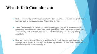
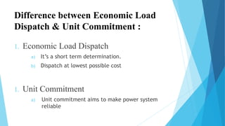
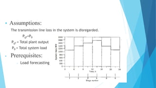
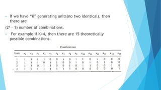
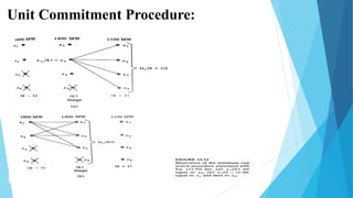
ECONOMIC OPERATION OF POWER 
SYSTEMS BY UNIT COMMITMENT 
Department Of Electrical And Electronics Engineering 
IIIT Bhubaneswar 
Bhubaneswar- 756003, Odisha
ECONOMIC OPERATION OF POWER 
SYSTEMS BY UNIT COMMITMENT 
Seminar presented by 
PRITESH PRIYADARSHI 
(B311029) 
under the guidance of 
Dr. P K RAY 
Department Of Electrical And Electronics Engineering 
IIIT Bhubaneswar
OUTLINE: 
1. Why Unit Commitment ? 
2. What is Unit commitment ? 
3. Difference between Economic Load Dispatch & Unit Commitment 
4. Unit Commitment Terminology 
5. Unit Commitment Procedure 
6. Solving The Unit Commitment Problem (Dynamic Programming)
Why Unit Commitment
What is Unit Commitment: 
 Unit commitment plans for best set of units to be available to supply the predicted or 
forecast load of the system over a future time period. 
 “Unit Commitment” is therefore, one way to suggest, just sufficient number of 
generating units with sufficient amount of generating capacity to meet a given load 
economically with sufficient reserve capacity to meet any abnormal, operating 
condition. 
 Here we consider the problem of scheduling fossil fired thermal units in which the 
aggregate costs( such as start up cost, operating fuel costs & shut down costs ) are to 
be minimized over a daily load cycle.
Difference between Economic Load 
Dispatch & Unit Commitment : 
1. Economic Load Dispatch 
a) It’s a short term determination. 
b) Dispatch at lowest possible cost 
1. Unit Commitment 
a) Unit commitment aims to make power system 
reliable
 Assumptions: 
The transmission line loss in the system is disregarded. 
PgT=PD 
PgT = Total plant output 
PD = Total system load 
 Prerequisites: 
 Load forecasting
 If we have “K” generating units(no two identical), then 
there are 
(2k – 1) number of combinations. 
 For example if K=4, then there are 15 theoretically 
possible combinations.
 Xi(k) = combination Xi of interval k 
 Pi(k) = minimum production cost of combination Xi(k) 
 Tij(k) = cost of transition from combination Xi(k) to combination Xj(k+1) 
between intervals k and k+1 
 Fij(k) = The cost associated with any stage k 
Fij(k) = Pi(k) + Tij(k)
Unit Commitment Procedure:
Dynamic Programming: 
 We use “Dynamic programming” to solve Unit Commitment problem. 
 Here we take an iterative relation embodying the principle that starting with 
given combination Xi* at stage k, the minimum unit commitment cost is found 
by minimizing the sum of the current single-stage cost fij(k) plus the minimum 
cumulative cost Fij(k+1) over the later stages of study. 
 This is one example of the principle of optimality, which states: if possible 
path from A to C passes through intermediate point B , then the best possible 
path from B to C must be corresponding part of the best path from A to C. 
 Computationally, we evaluate one decision at a time beginning with the final 
stage N and carry the minimum cumulative cost function backward in time to 
stage k to find the minimum cumulative cost Fi*(k) for the feasible 
combination.
Contd. 
 The minimum cumulative cost decisions are recovered as we sweep from stage 1 
to stage N searching through the tables already calculated for each stage. This 
computational procedure is known as Dynamic Programming.2 
 It involves two sweeps through each stage k. 
 In the first sweep, which is computationally intensive, we work backward 
computing and recording for each candidate combination xi of stage k the 
minimum Fi(k) and its associated xj(k+1). 
 The second sweep in the forward direction does not involve any processing since 
with xi*(k) identified we merely enter the table of results already recorded to 
retrieve the value Fi*(k) and its associated combination xj(k+1), which becomes 
xi*(k+1) as we move to next forward stage.
References: 
 “Power system Analysis” by John J. Grainger, William D. Stevenson 
 R. Bellman, Dynamic Programming, Princeton University Press, Princeton, NJ, 
1957.
Economic operation of Power systems by Unit commitment

Economic operation of Power systems by Unit commitment

  • 1.
    ECONOMIC OPERATION OFPOWER SYSTEMS BY UNIT COMMITMENT Department Of Electrical And Electronics Engineering IIIT Bhubaneswar Bhubaneswar- 756003, Odisha
  • 2.
    ECONOMIC OPERATION OFPOWER SYSTEMS BY UNIT COMMITMENT Seminar presented by PRITESH PRIYADARSHI (B311029) under the guidance of Dr. P K RAY Department Of Electrical And Electronics Engineering IIIT Bhubaneswar
  • 3.
    OUTLINE: 1. WhyUnit Commitment ? 2. What is Unit commitment ? 3. Difference between Economic Load Dispatch & Unit Commitment 4. Unit Commitment Terminology 5. Unit Commitment Procedure 6. Solving The Unit Commitment Problem (Dynamic Programming)
  • 4.
  • 5.
    What is UnitCommitment:  Unit commitment plans for best set of units to be available to supply the predicted or forecast load of the system over a future time period.  “Unit Commitment” is therefore, one way to suggest, just sufficient number of generating units with sufficient amount of generating capacity to meet a given load economically with sufficient reserve capacity to meet any abnormal, operating condition.  Here we consider the problem of scheduling fossil fired thermal units in which the aggregate costs( such as start up cost, operating fuel costs & shut down costs ) are to be minimized over a daily load cycle.
  • 6.
    Difference between EconomicLoad Dispatch & Unit Commitment : 1. Economic Load Dispatch a) It’s a short term determination. b) Dispatch at lowest possible cost 1. Unit Commitment a) Unit commitment aims to make power system reliable
  • 7.
     Assumptions: Thetransmission line loss in the system is disregarded. PgT=PD PgT = Total plant output PD = Total system load  Prerequisites:  Load forecasting
  • 8.
     If wehave “K” generating units(no two identical), then there are (2k – 1) number of combinations.  For example if K=4, then there are 15 theoretically possible combinations.
  • 9.
     Xi(k) =combination Xi of interval k  Pi(k) = minimum production cost of combination Xi(k)  Tij(k) = cost of transition from combination Xi(k) to combination Xj(k+1) between intervals k and k+1  Fij(k) = The cost associated with any stage k Fij(k) = Pi(k) + Tij(k)
  • 10.
  • 11.
    Dynamic Programming: We use “Dynamic programming” to solve Unit Commitment problem.  Here we take an iterative relation embodying the principle that starting with given combination Xi* at stage k, the minimum unit commitment cost is found by minimizing the sum of the current single-stage cost fij(k) plus the minimum cumulative cost Fij(k+1) over the later stages of study.  This is one example of the principle of optimality, which states: if possible path from A to C passes through intermediate point B , then the best possible path from B to C must be corresponding part of the best path from A to C.  Computationally, we evaluate one decision at a time beginning with the final stage N and carry the minimum cumulative cost function backward in time to stage k to find the minimum cumulative cost Fi*(k) for the feasible combination.
  • 12.
    Contd.  Theminimum cumulative cost decisions are recovered as we sweep from stage 1 to stage N searching through the tables already calculated for each stage. This computational procedure is known as Dynamic Programming.2  It involves two sweeps through each stage k.  In the first sweep, which is computationally intensive, we work backward computing and recording for each candidate combination xi of stage k the minimum Fi(k) and its associated xj(k+1).  The second sweep in the forward direction does not involve any processing since with xi*(k) identified we merely enter the table of results already recorded to retrieve the value Fi*(k) and its associated combination xj(k+1), which becomes xi*(k+1) as we move to next forward stage.
  • 14.
    References:  “Powersystem Analysis” by John J. Grainger, William D. Stevenson  R. Bellman, Dynamic Programming, Princeton University Press, Princeton, NJ, 1957.