This program solves the economic dispatch problem using the lambda iteration method for a system with three generating units, both with and without considering transmission losses. It defines the cost curves and operating limits of each generator. The problem is solved by minimizing total generation cost subject to the load demand constraint, using MATLAB's fsolve function to solve the coordination equations. Without losses, it calculates the optimal dispatch, total cost and verifies load balance. With losses, it iteratively solves the coordination equations including loss coefficients to determine the optimal dispatch that minimizes total cost including losses, calculating total losses and resulting load supplied.

1. Project on Economic Load dispatch

2. Economic Load dispatchWhat is economic dispatch?The definition of economic dispatch is:“The operation of generation facilities to produce energy at the lowest cost to reliably serve consumers, recognizing any operational limits of generation and transmission facilities”. Most electric power systems dispatch their own generating units and their own purchased power in a way that may be said to meet this definition.The factors influencing power generation at minimum cost are :operating efficiencies of generators

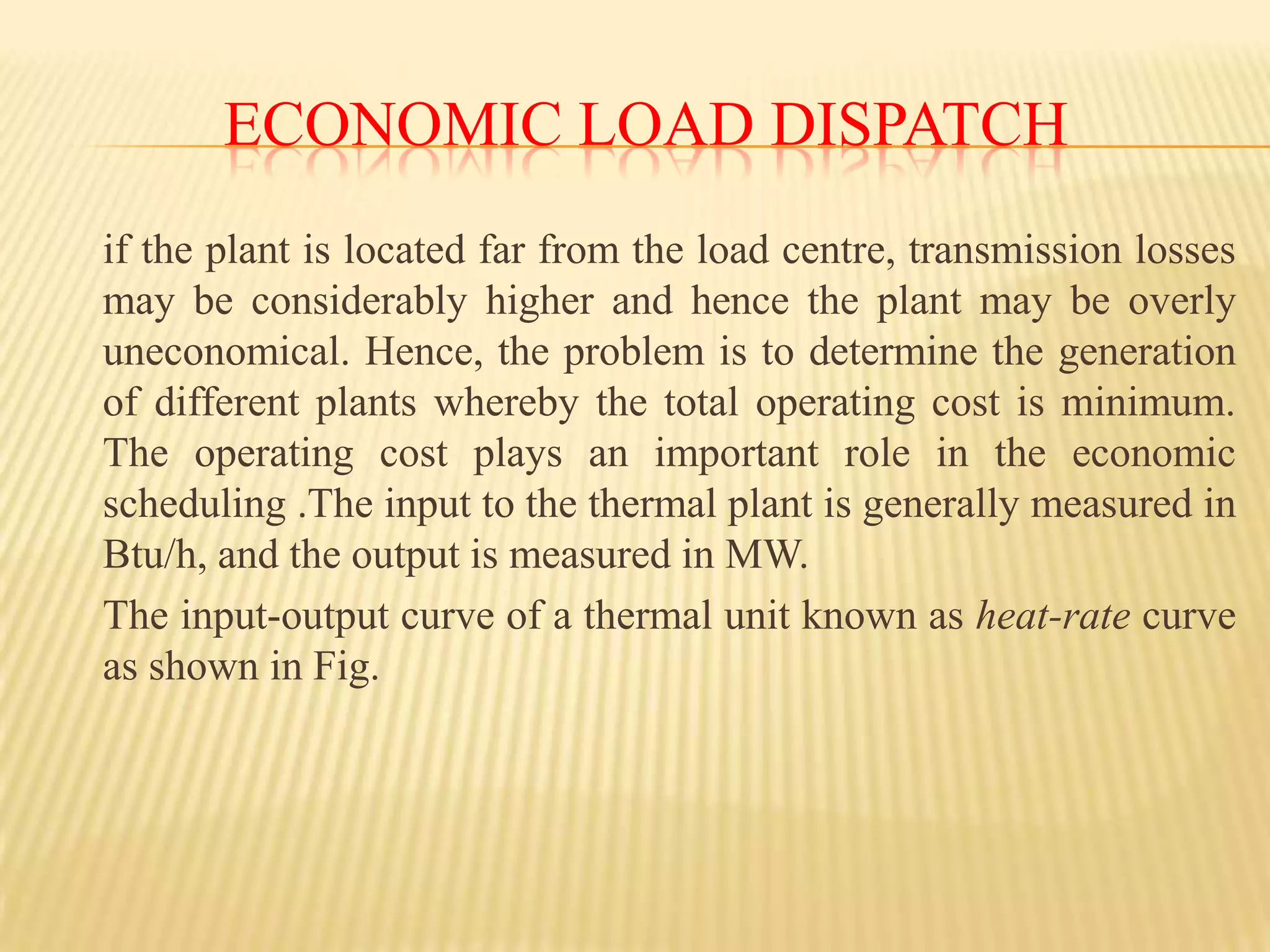
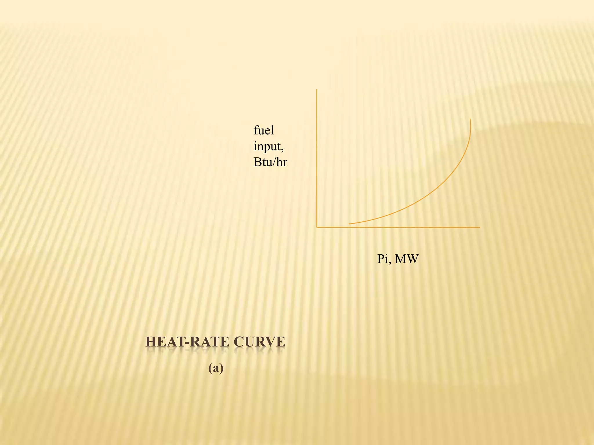
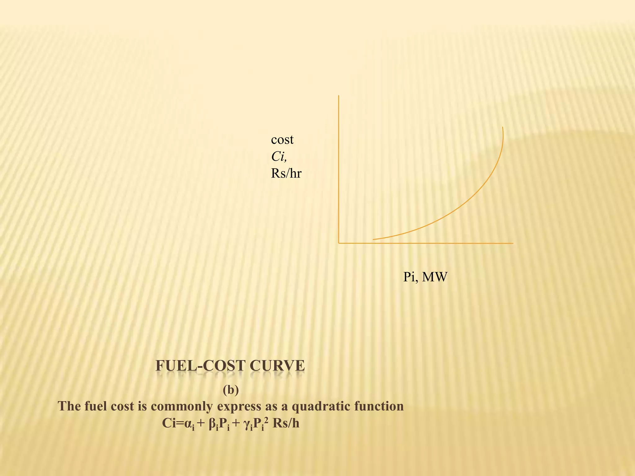
3. fuel cost and transmission lossesEconomic Load dispatch if the plant is located far from the load centre, transmission losses may be considerably higher and hence the plant may be overly uneconomical. Hence, the problem is to determine the generation of different plants whereby the total operating cost is minimum. The operating cost plays an important role in the economic scheduling .The input to the thermal plant is generally measured in Btu/h, and the output is measured in MW.The input-output curve of a thermal unit known as heat-rate curve as shown in Fig.

4. Heat-Rate Curve(a)fuelinput,Btu/hrPi, MW

5. Fuel-Cost Curve(b)The fuel cost is commonly express as a quadratic functionCi=αi+ βiPi+ γiPi2 Rs/h costCi,Rs/hrPi, MW

6. incremental fuel-cost curveThe derivative is known as the incremental fuel cost.λRs/MWhPi, MW

7. Economic Load dispatchAn economic dispatch schedule for assigning loads to each unit in a plant can be prepared by assuming various values of total plant output

8. calculating the corresponding incremental fuel cost λ of the plant

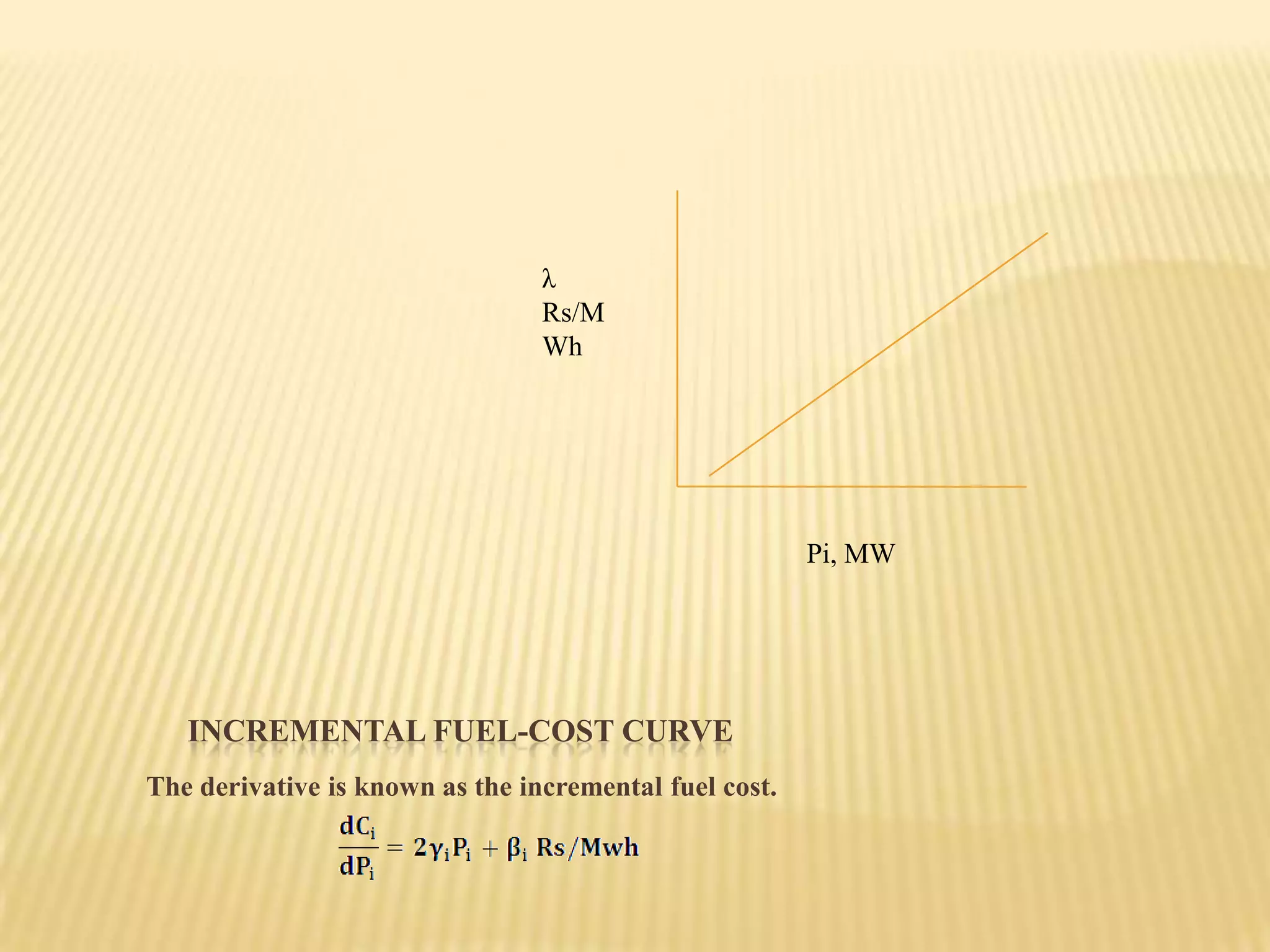
9. substituting the value of λ for λi in the equation for the incremental fuel cost of each unit to calculate its output. For a plant with two units having no transmission losses operating under economic load distribution the λ of the plant equals λi of each unit, and soλ= dC1/dP1 = 2γ1 P1+β1 ; λ= dC2/dP2 = 2γ2 P2+β2;and

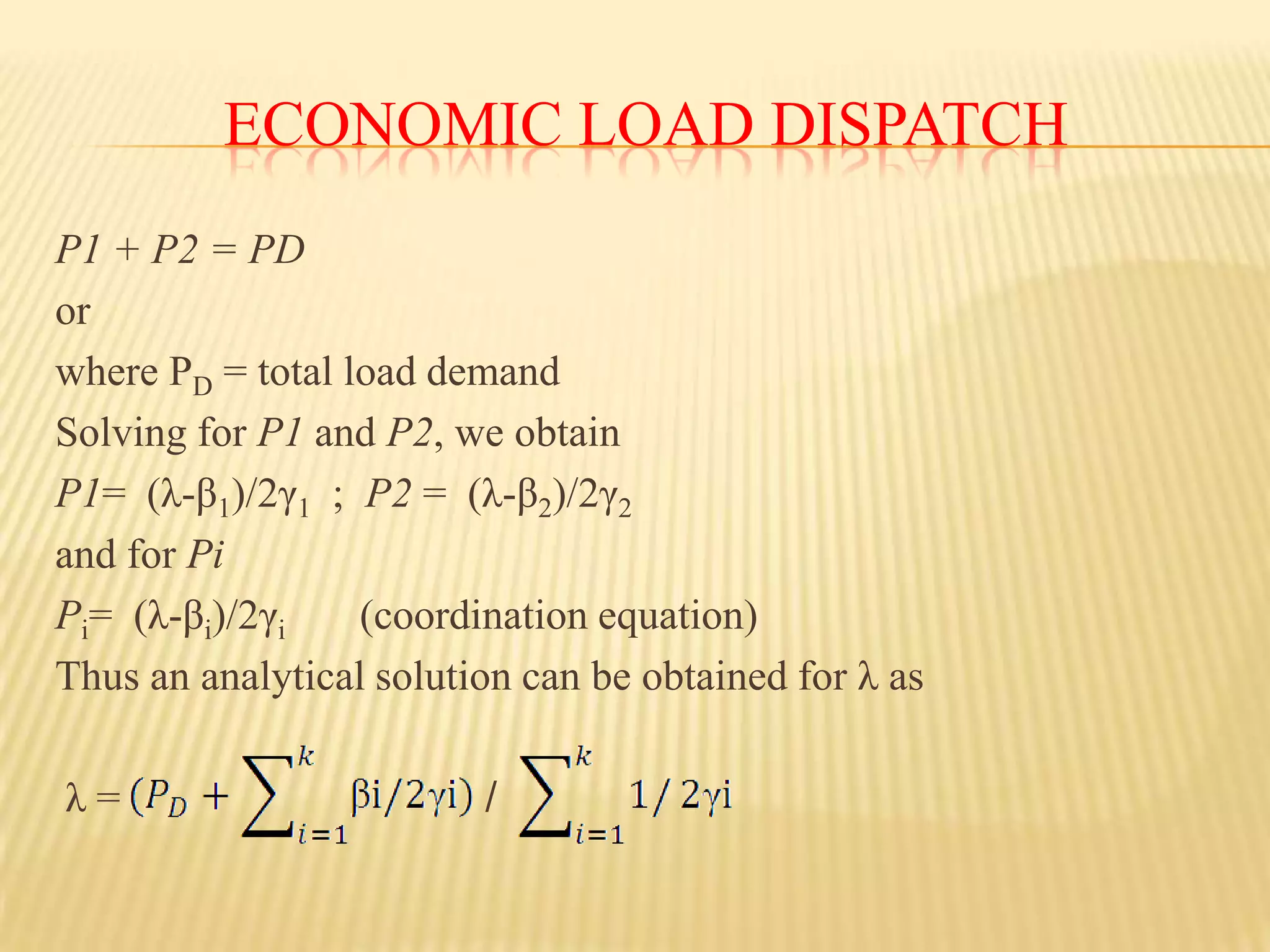
10. Economic Load dispatchP1 + P2 = PD or where PD= total load demandSolving for P1 and P2, we obtainP1= (λ-β1)/2γ1 ; P2 = (λ-β2)/2γ2 and for PiPi= (λ-βi)/2γi (coordination equation) Thus an analytical solution can be obtained for λ as λ = /

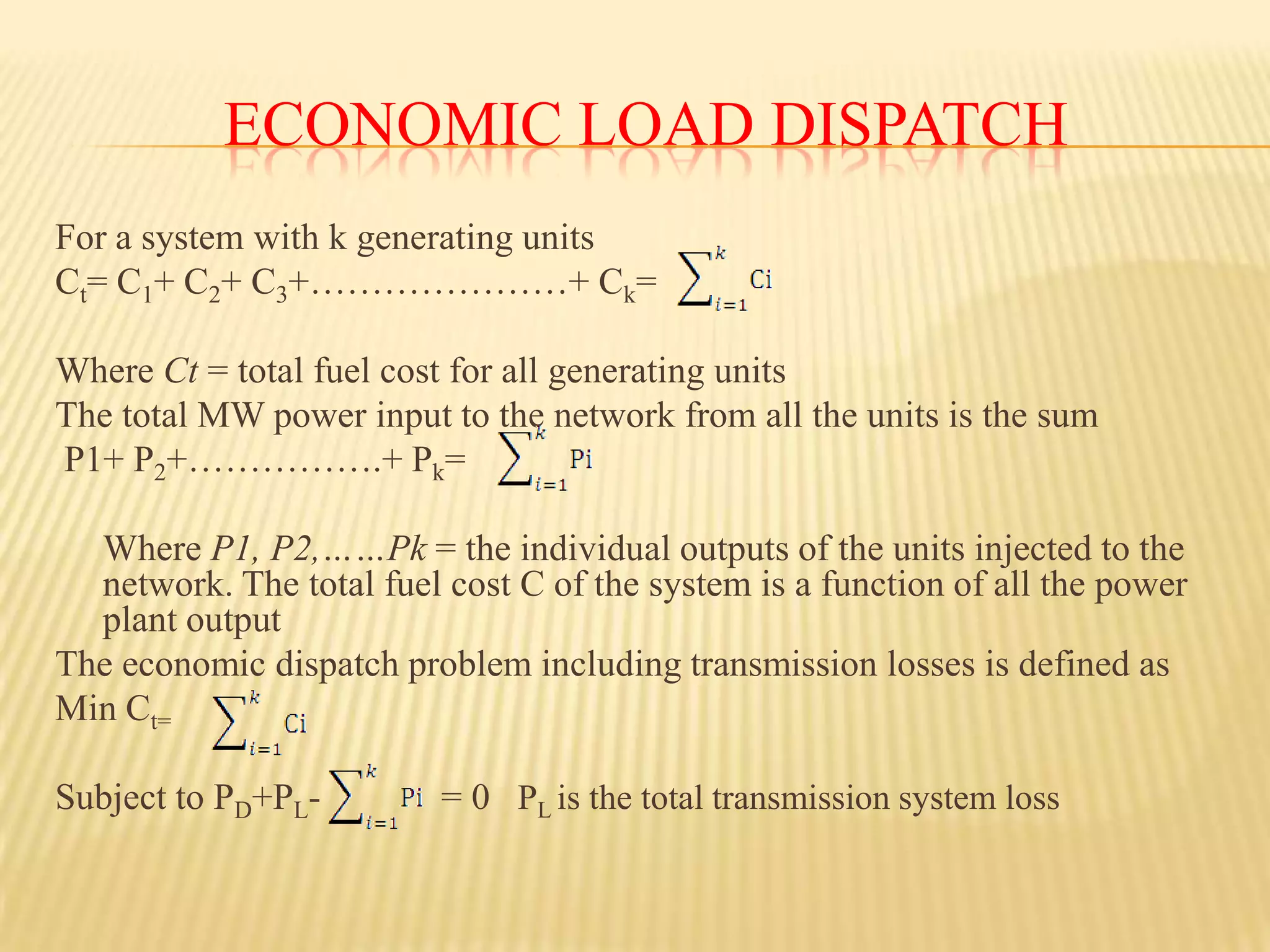
11. Economic Load dispatchFor a system with k generating units Ct= C1+ C2+ C3+…………………+ Ck= Where Ct = total fuel cost for all generating units The total MW power input to the network from all the units is the sum P1+P2+…………….+Pk= Where P1, P2,……Pk= the individual outputs of the units injected to the network. The total fuel cost C of the system is a function of all the power plant output The economic dispatch problem including transmission losses is defined asMin Ct=Subject to PD+PL- = 0 PL is the total transmission system loss

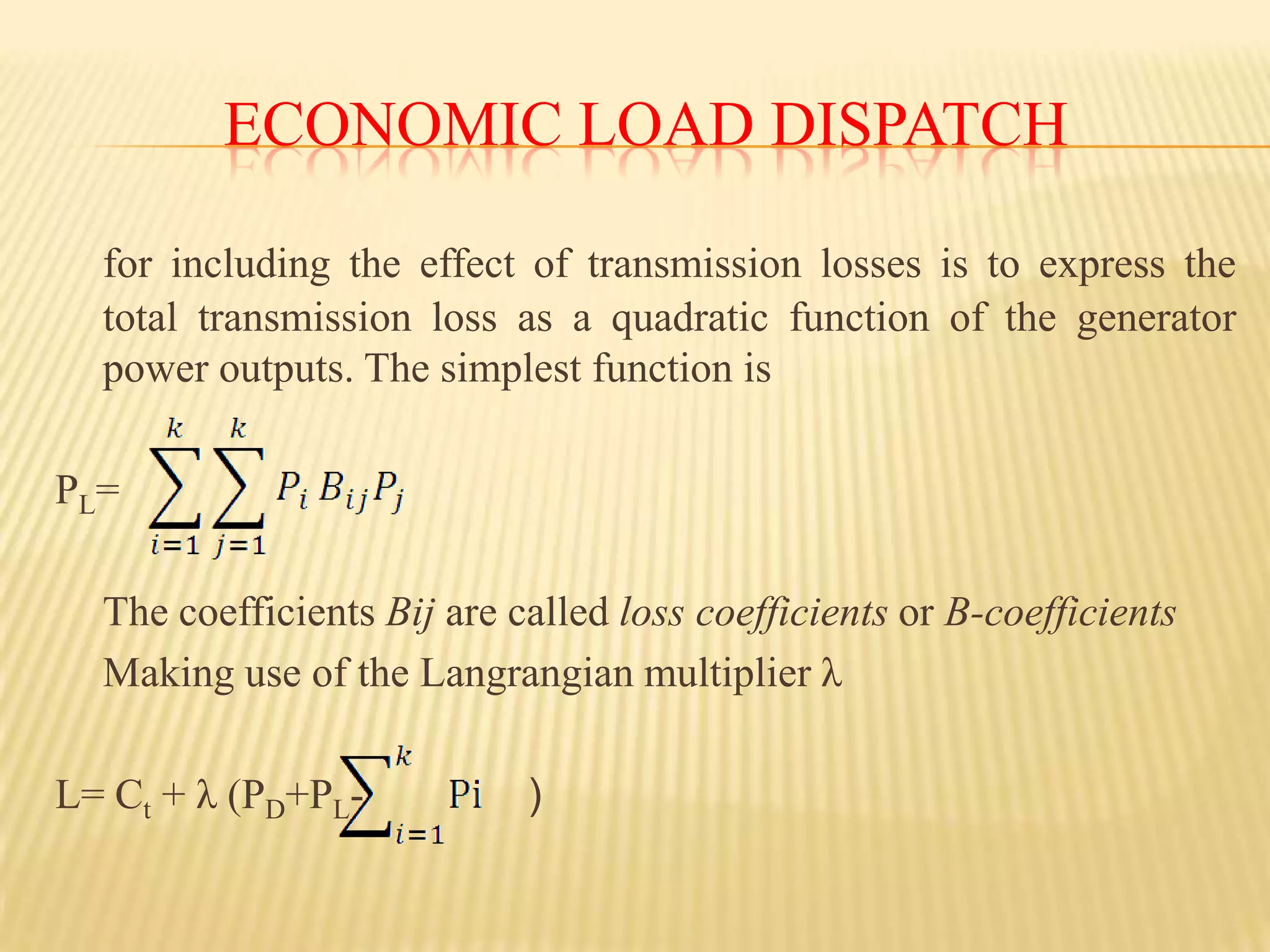
12. Economic Load dispatchfor including the effect of transmission losses is to express the total transmission loss as a quadratic function of the generator power outputs. The simplest function isPL= The coefficients Bijare called loss coefficients or B-coefficients Making use of the Langrangian multiplier λ L= Ct + λ (PD+PL- )

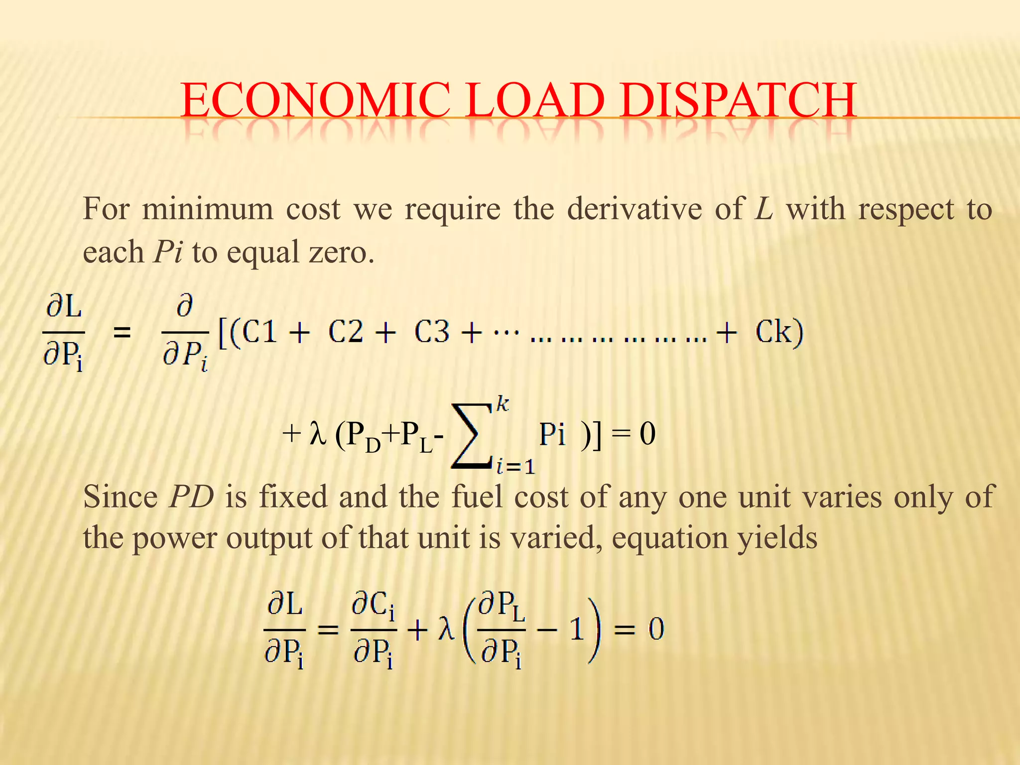
13. Economic Load dispatchFor minimum cost we require the derivative of L with respect to each Pi to equal zero. Since PD is fixed and the fuel cost of any one unit varies only of the power output of that unit is varied, equation yields=+ λ (PD+PL- )] = 0

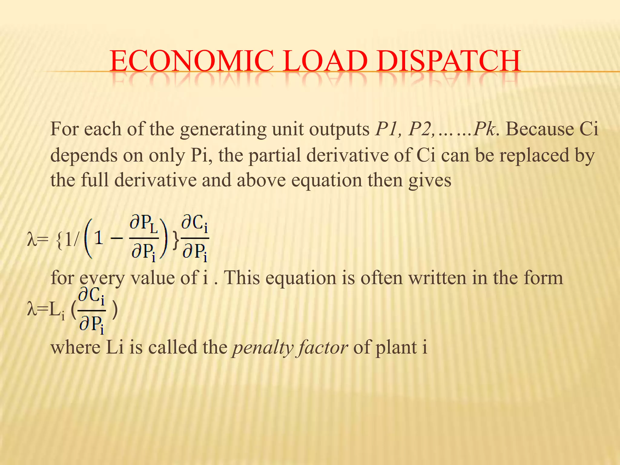
14. Economic Load dispatchFor each of the generating unit outputs P1, P2,……Pk. Because Ci depends on only Pi, the partial derivative of Ci can be replaced by the full derivative and above equation then gives λ= {1/ }for every value of i . This equation is often written in the formλ=Li( )where Li is called the penalty factor of plant i

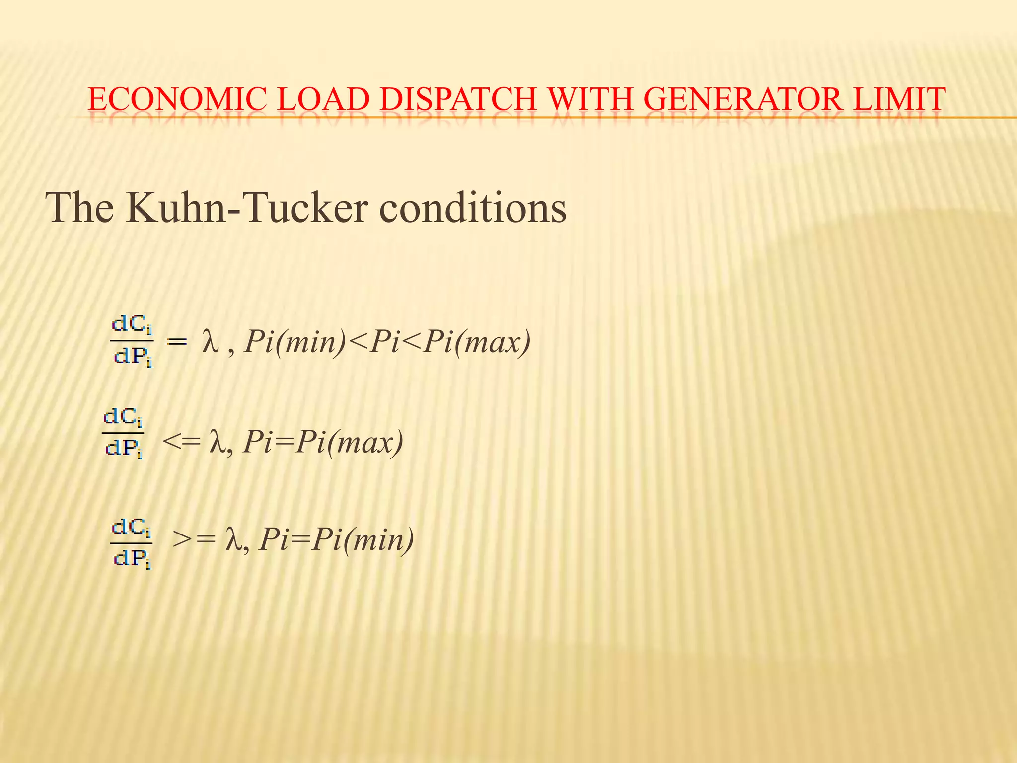
15. Economic Load dispatch with generator limitThe power output of any generator should not exceed its rating nor be below the value for stable boiler operationGenerators have a minimum and maximum real power output limits.

16. The problem is to find the real power generation for each plant such that cost are minimized, subject to:

17. Meeting load demand - equality constraints

18. Constrained by the generator limits - inequality constraintsEconomic Load dispatch with generator limitThe Kuhn-Tucker conditionsλ , Pi(min)<Pi<Pi(max) <= λ, Pi=Pi(max) >= λ, Pi=Pi(min)

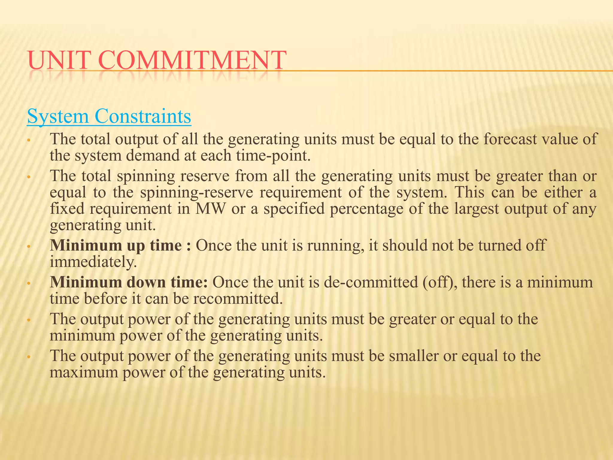
19. Unit commitmentSystem ConstraintsThe total outputof all the generating units must be equal tothe forecast value of the system demandat each time-point.

20. The total spinning reservefrom all the generating units must be greater than or equal to the spinning-reserve requirement of the system. This can be either a fixed requirement in MW or a specified percentage of the largest output of any generating unit.

21. Minimum up time : Once the unit is running, it should not be turned off immediately.

22. Minimum down time: Once the unit is de-committed (off), there is a minimum time before it can be recommitted.

23. The output powerof the generating units must be greater or equalto the minimum powerof the generating units.

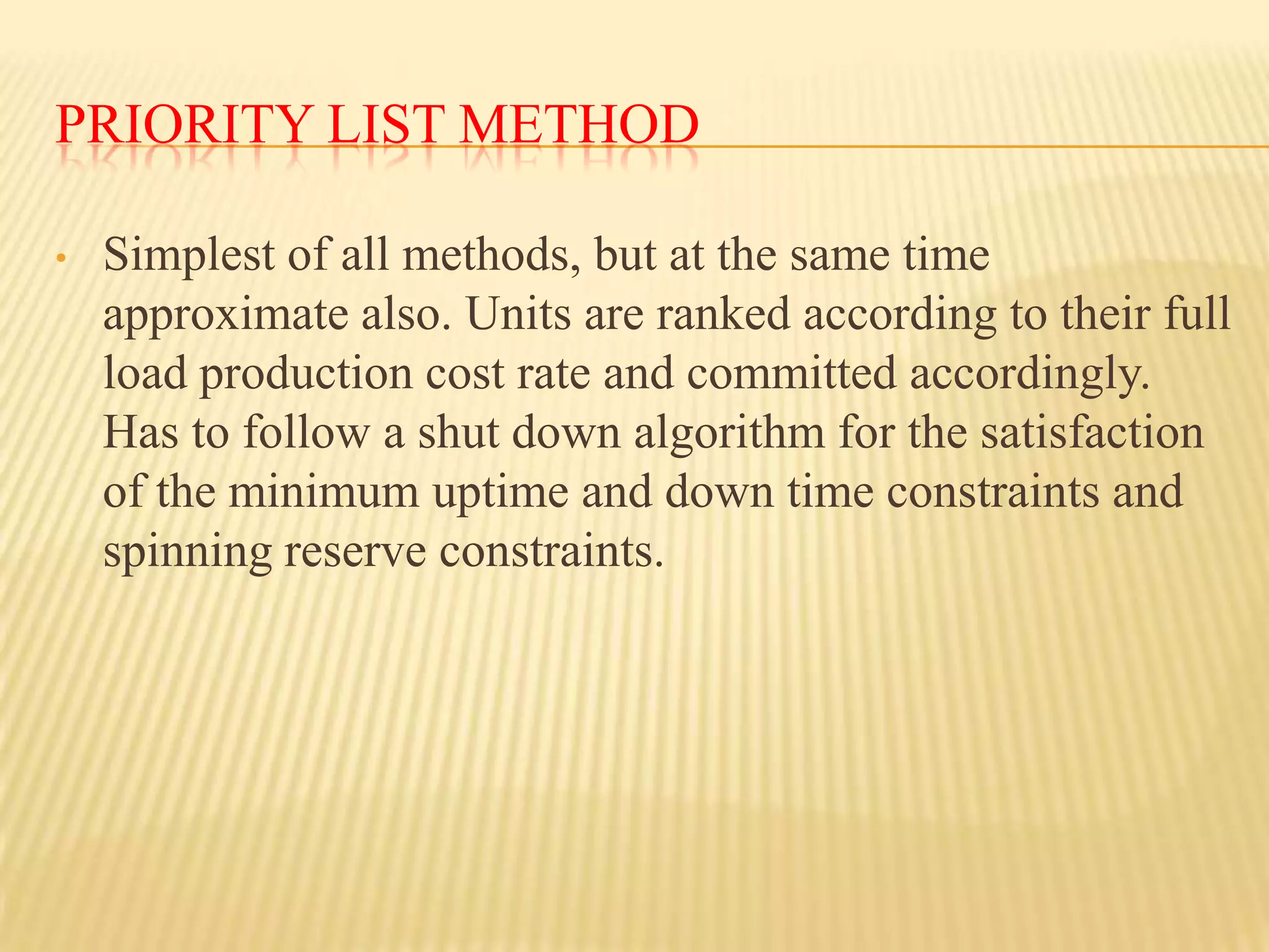
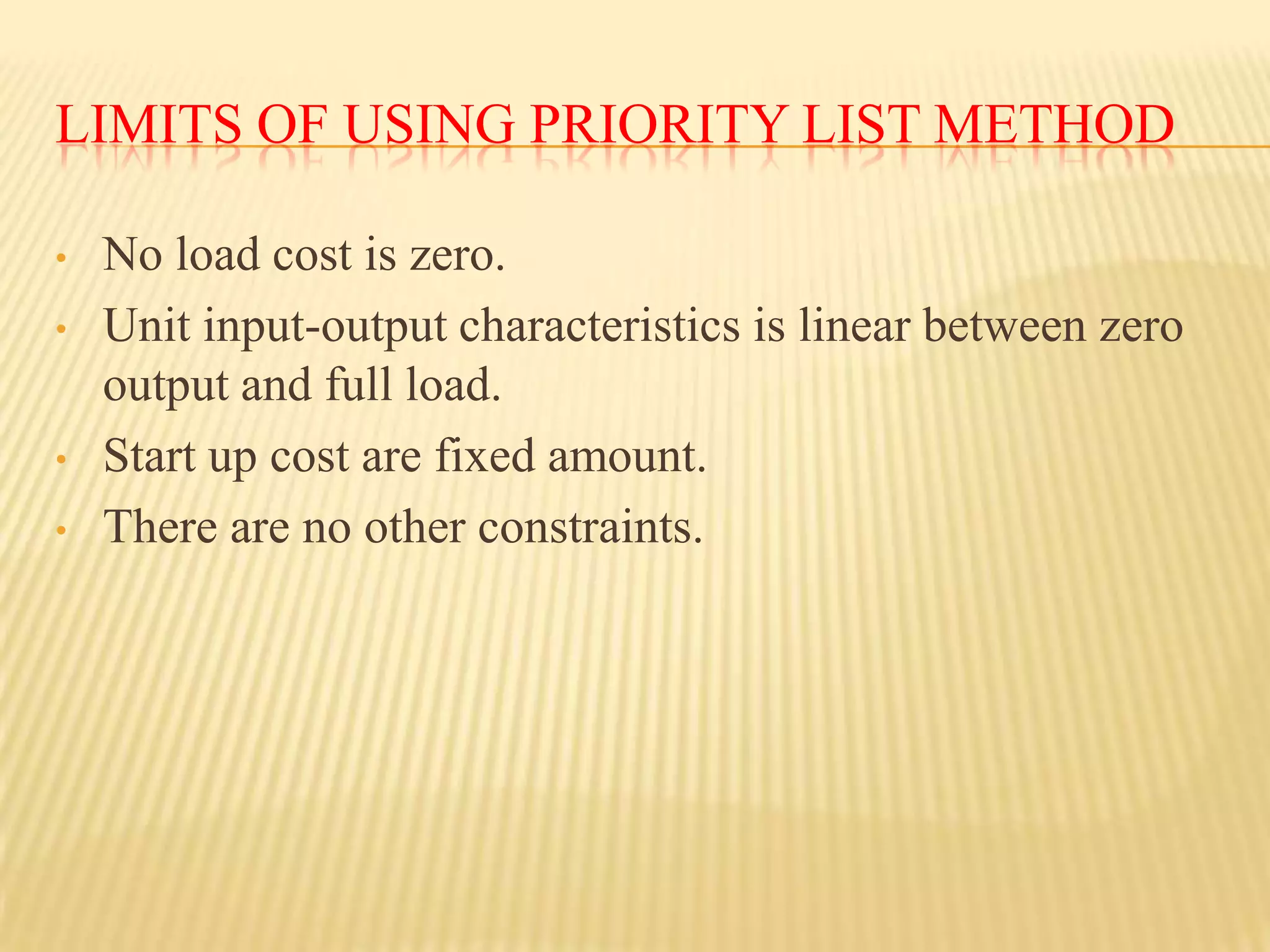
24. The output powerof the generating units must be smaller or equalto the maximum powerof the generating units.Priority list methodSimplest of all methods, but at the same time approximate also. Units are ranked according to their full load production cost rate and committed accordingly. Has to follow a shut down algorithm for the satisfaction of the minimum uptime and down time constraints and spinning reserve constraints.limits of using priority list methodNo load cost is zero.

25. Unit input-output characteristics is linear between zero output and full load.

26. Start up cost are fixed amount.

27. There are no other constraints.

28. Economic Dispatch – SummaryEconomic dispatch determines the best way to minimize the current generator operating costs.

29. The lambda-iteration method is a good approach for solving the economic dispatch problem.

30. generator limits are easily handled

31. penalty factors are used to consider the impact of losses

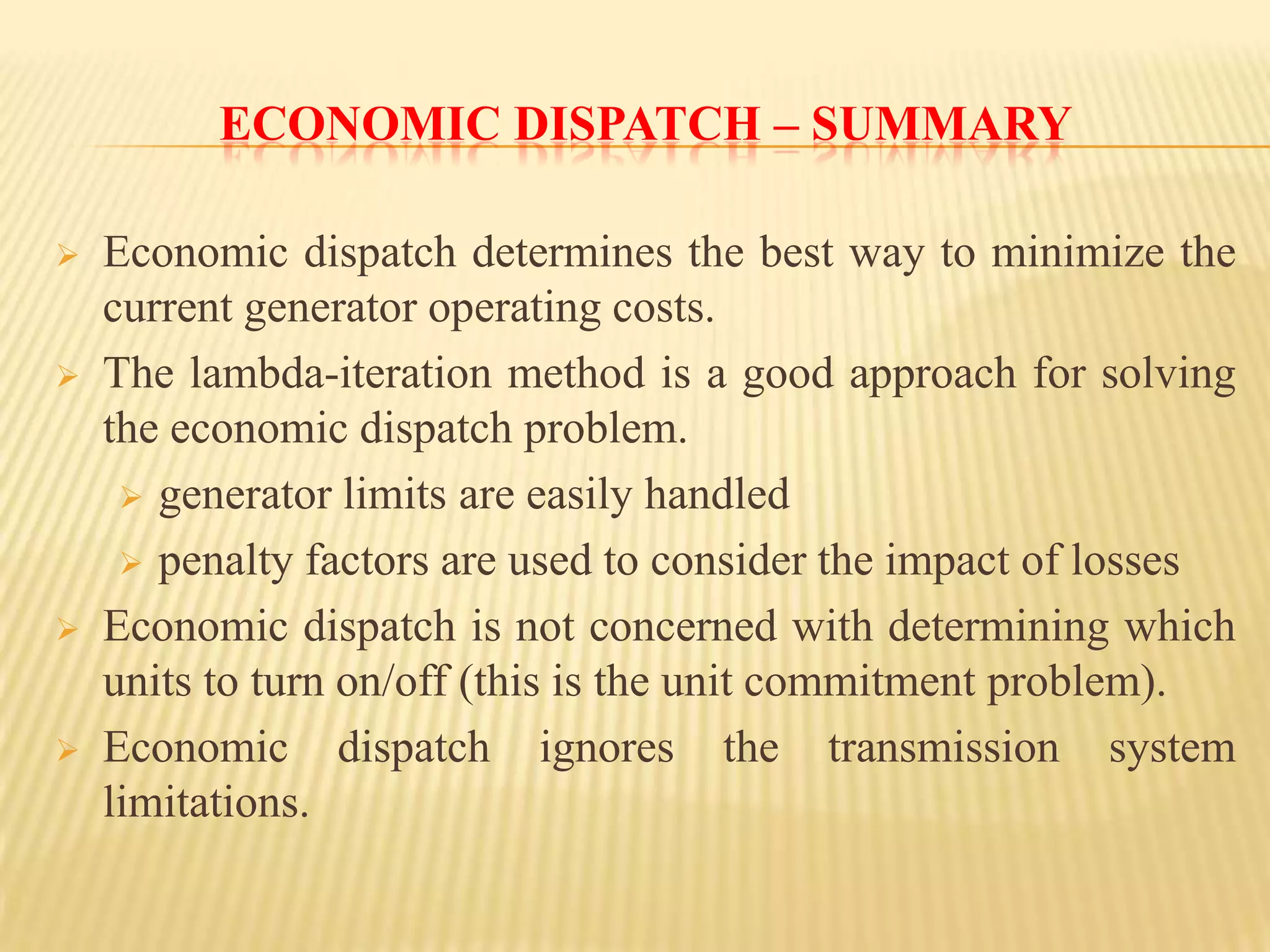
32. Economic dispatch is not concerned with determining which units to turn on/off (this is the unit commitment problem).

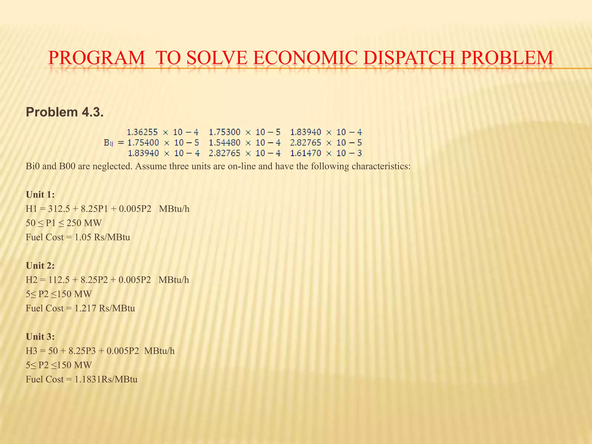
33. Economic dispatch ignores the transmission system limitations.program to solve economic dispatch problem Problem 4.3.Bi0 and B00 are neglected. Assume three units are on-line and have the following characteristics: Unit 1: H1 = 312.5 + 8.25P1 + 0.005P2 MBtu/h50 ≤ P1 ≤ 250 MWFuel Cost = 1.05 Rs/MBtu Unit 2: H2 = 112.5 + 8.25P2 + 0.005P2 MBtu/h5≤ P2 ≤150 MWFuel Cost = 1.217 Rs/MBtu Unit 3: H3 = 50 + 8.25P3 + 0.005P2 MBtu/h5≤ P2 ≤150 MWFuel Cost = 1.1831Rs/MBtu

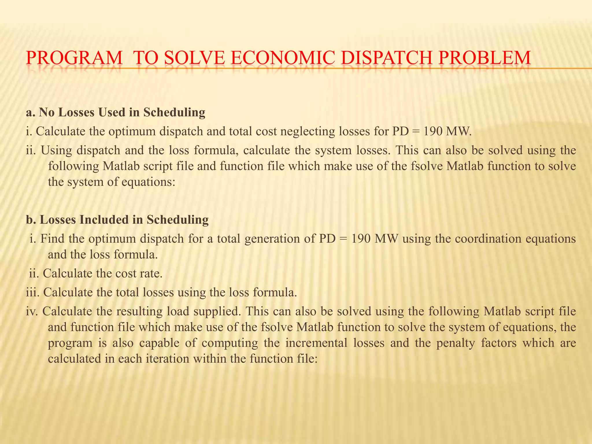
34. program to solve economic dispatch problem a. No Losses Used in Scheduling i. Calculate the optimum dispatch and total cost neglecting losses for PD = 190 MW. ii. Using dispatch and the loss formula, calculate the system losses. This can also be solved using the following Matlab script file and function file which make use of the fsolveMatlab function to solve the system of equations:b. Losses Included in Scheduling i. Find the optimum dispatch for a total generation of PD = 190 MW using the coordination equations and the loss formula. ii. Calculate the cost rate. iii. Calculate the total losses using the loss formula. iv. Calculate the resulting load supplied. This can also be solved using the following Matlab script file and function file which make use of the fsolveMatlab function to solve the system of equations, the program is also capable of computing the incremental losses and the penalty factors which are calculated in each iteration within the function file:

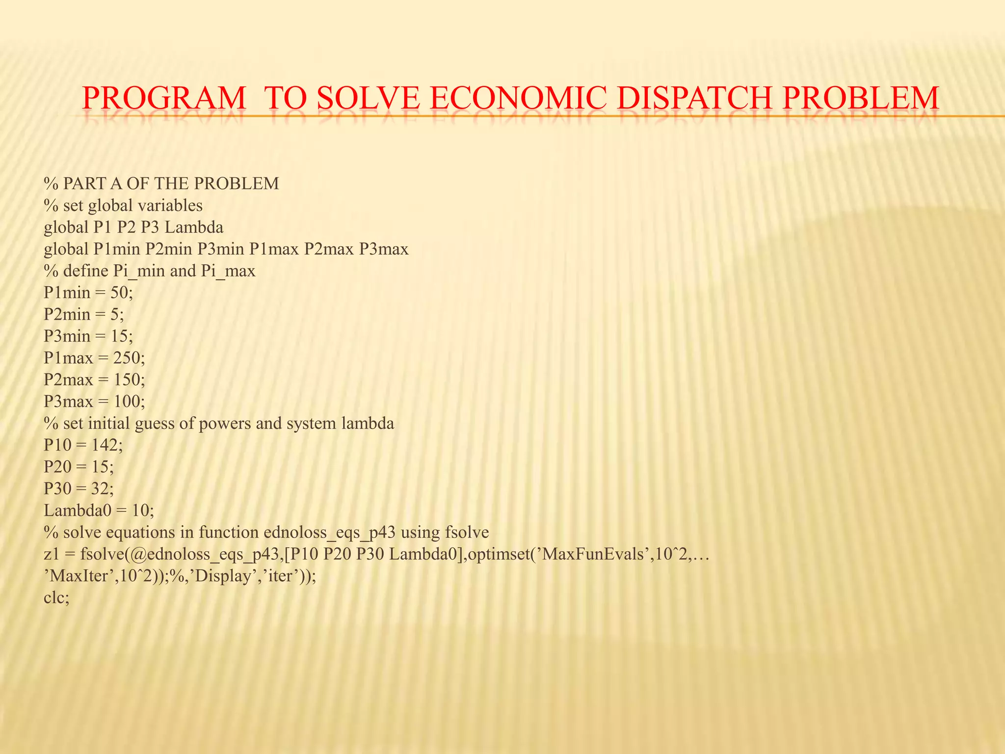
35. program to solve economic dispatch problem % PART A OF THE PROBLEM% set global variablesglobal P1 P2 P3 Lambdaglobal P1min P2min P3min P1max P2max P3max% define Pi_min and Pi_maxP1min = 50;P2min = 5;P3min = 15;P1max = 250;P2max = 150;P3max = 100;% set initial guess of powers and system lambdaP10 = 142;P20 = 15;P30 = 32;Lambda0 = 10;% solve equations in function ednoloss_eqs_p43 using fsolvez1 = fsolve(@ednoloss_eqs_p43,[P10 P20 P30 Lambda0],optimset(’MaxFunEvals’,10ˆ2,…’MaxIter’,10ˆ2));%,’Display’,’iter’));clc;

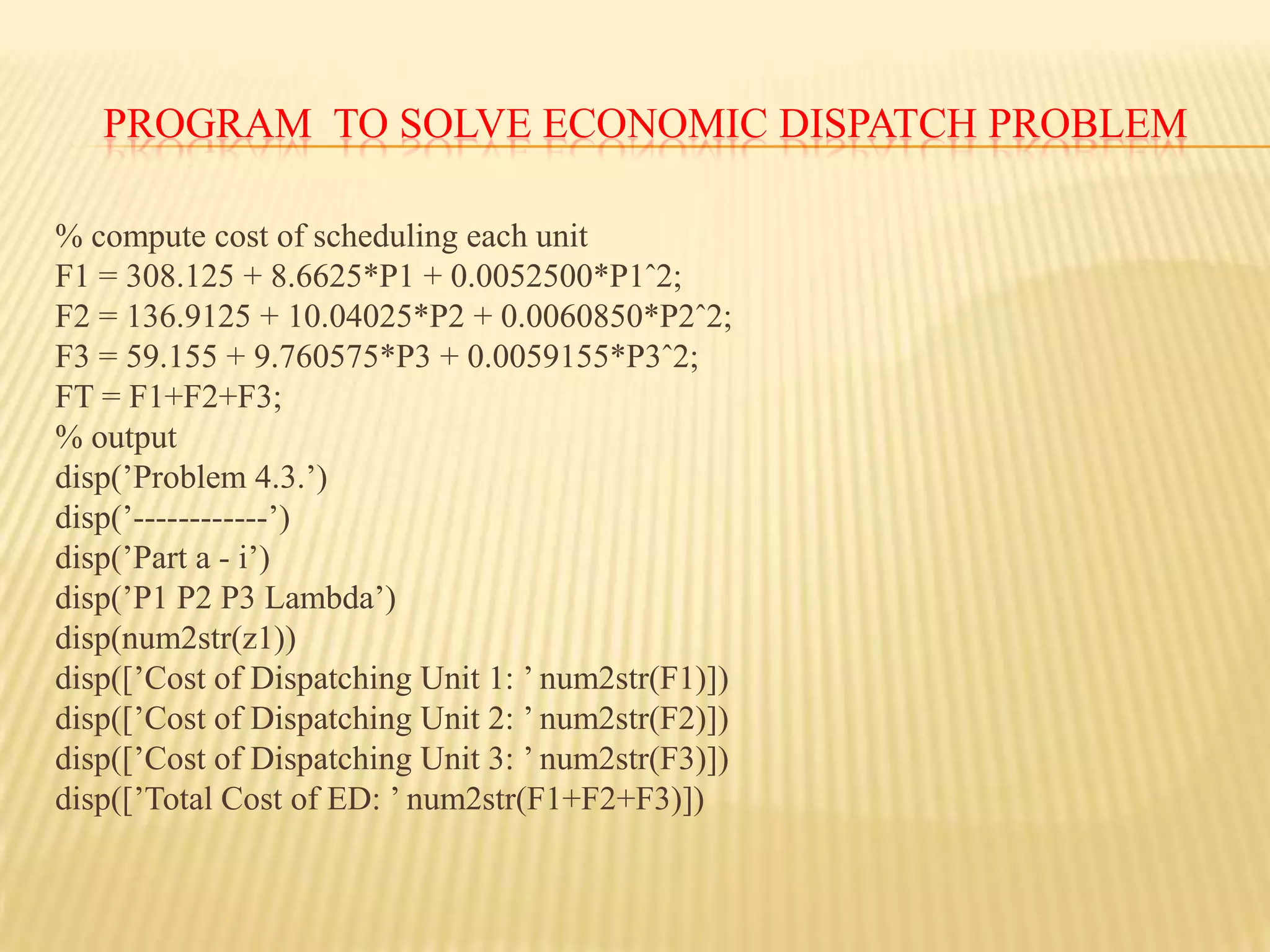
36. program to solve economic dispatch problem % compute cost of scheduling each unitF1 = 308.125 + 8.6625*P1 + 0.0052500*P1ˆ2;F2 = 136.9125 + 10.04025*P2 + 0.0060850*P2ˆ2;F3 = 59.155 + 9.760575*P3 + 0.0059155*P3ˆ2;FT = F1+F2+F3;% outputdisp(’Problem 4.3.’)disp(’------------’)disp(’Part a - i’)disp(’P1 P2 P3 Lambda’)disp(num2str(z1))disp([’Cost of Dispatching Unit 1: ’ num2str(F1)])disp([’Cost of Dispatching Unit 2: ’ num2str(F2)])disp([’Cost of Dispatching Unit 3: ’ num2str(F3)])disp([’Total Cost of ED: ’ num2str(F1+F2+F3)])

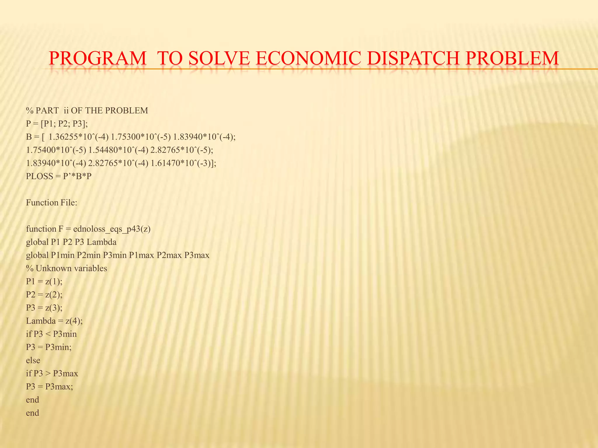
37. program to solve economic dispatch problem % PART ii OF THE PROBLEMP = [P1; P2; P3];B = [ 1.36255*10ˆ(-4) 1.75300*10ˆ(-5) 1.83940*10ˆ(-4);1.75400*10ˆ(-5) 1.54480*10ˆ(-4) 2.82765*10ˆ(-5);1.83940*10ˆ(-4) 2.82765*10ˆ(-4) 1.61470*10ˆ(-3)];PLOSS = P’*B*P Function File: function F = ednoloss_eqs_p43(z)global P1 P2 P3 Lambdaglobal P1min P2min P3min P1max P2max P3max% Unknown variablesP1 = z(1);P2 = z(2);P3 = z(3);Lambda = z(4);if P3 < P3minP3 = P3min;elseif P3 > P3maxP3 = P3max;endend

38. program to solve economic dispatch problem if P2 < P2minP2 = P2min;elseif P2 > P2maxP2 = P2max;endendif P1 < P1minP1 = P1min;elseif P1 > P1maxP1 = P1max;endend% dL/dPi and dL/dLambdaF(1,1) = 8.6625 + 0.0105*P1 - Lambda;F(2,1) = 10.04025 + 0.01217*P2 - Lambda;F(3,1) = 9.760575 + 0.011831*P3 - Lambda;F(4,1) = P1 + P2 + P3 - 190;

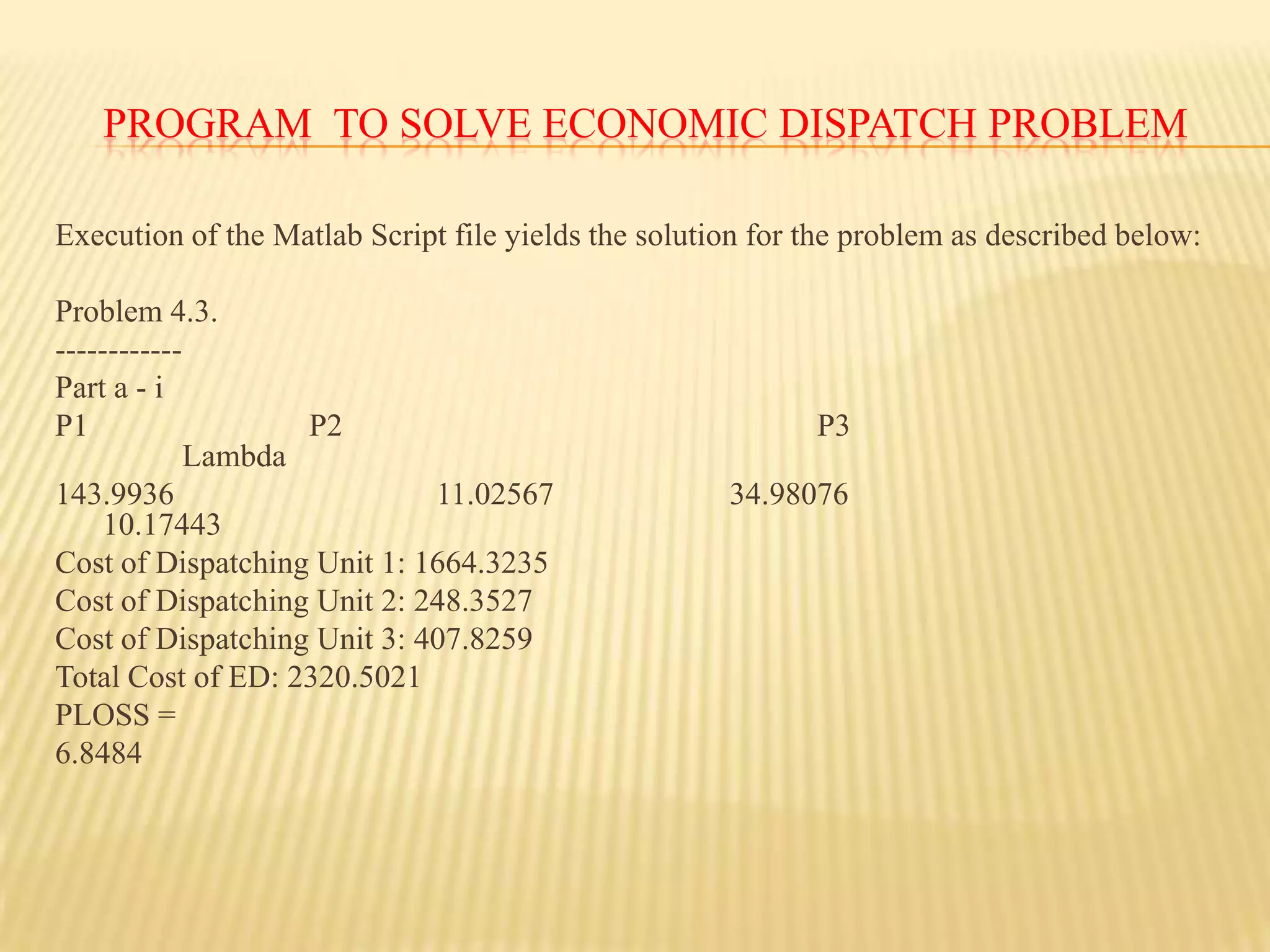
39. program to solve economic dispatch problem Execution of the Matlab Script file yields the solution for the problem as described below: Problem 4.3.------------Part a - iP1 P2 P3 Lambda143.9936 11.02567 34.98076 10.17443Cost of Dispatching Unit 1: 1664.3235Cost of Dispatching Unit 2: 248.3527Cost of Dispatching Unit 3: 407.8259Total Cost of ED: 2320.5021PLOSS =6.8484

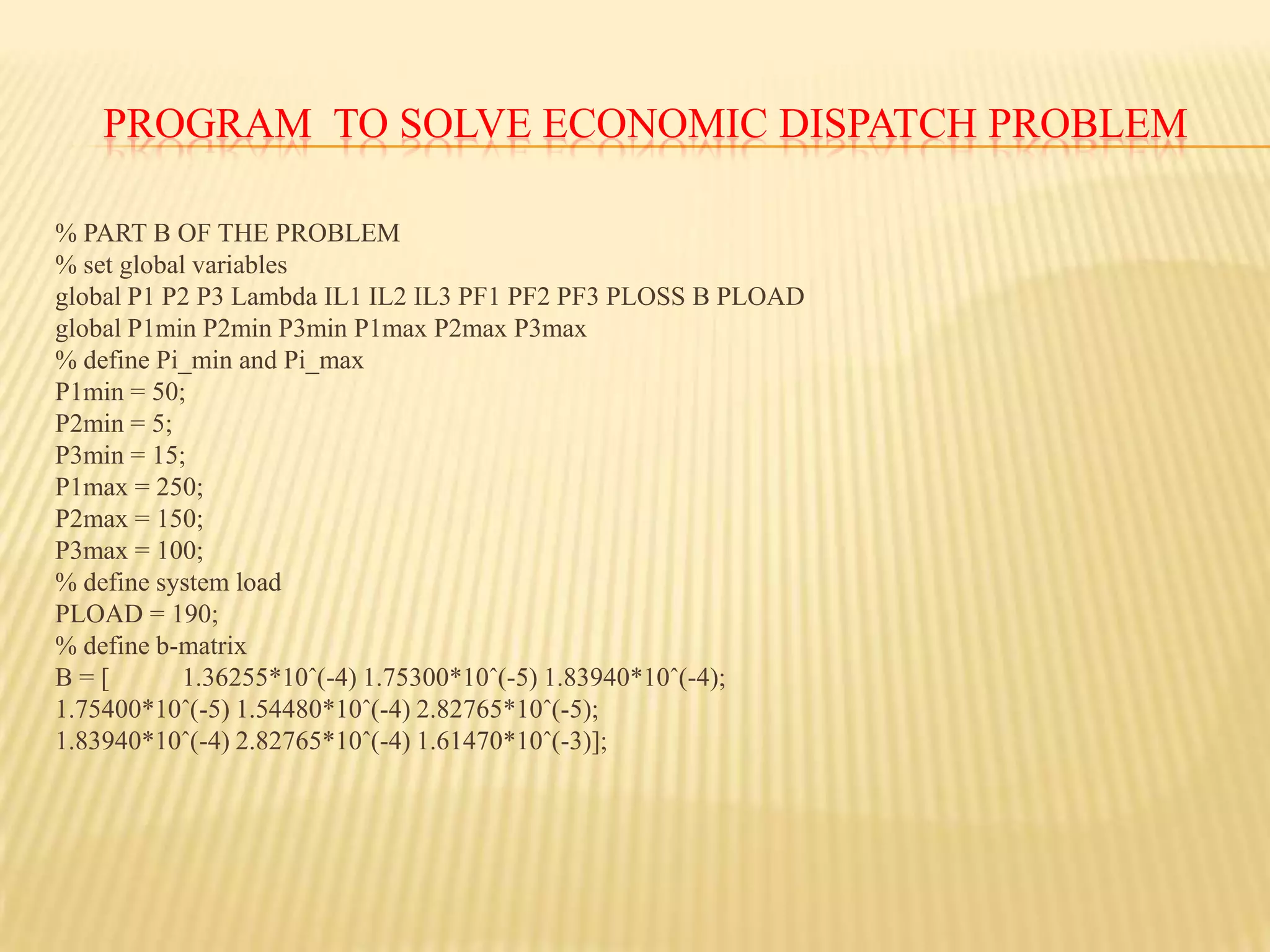
40. program to solve economic dispatch problem % PART B OF THE PROBLEM% set global variablesglobal P1 P2 P3 Lambda IL1 IL2 IL3 PF1 PF2 PF3 PLOSS B PLOADglobal P1min P2min P3min P1max P2max P3max% define Pi_min and Pi_maxP1min = 50;P2min = 5;P3min = 15;P1max = 250;P2max = 150;P3max = 100;% define system loadPLOAD = 190;% define b-matrixB = [ 1.36255*10ˆ(-4) 1.75300*10ˆ(-5) 1.83940*10ˆ(-4);1.75400*10ˆ(-5) 1.54480*10ˆ(-4) 2.82765*10ˆ(-5);1.83940*10ˆ(-4) 2.82765*10ˆ(-4) 1.61470*10ˆ(-3)];

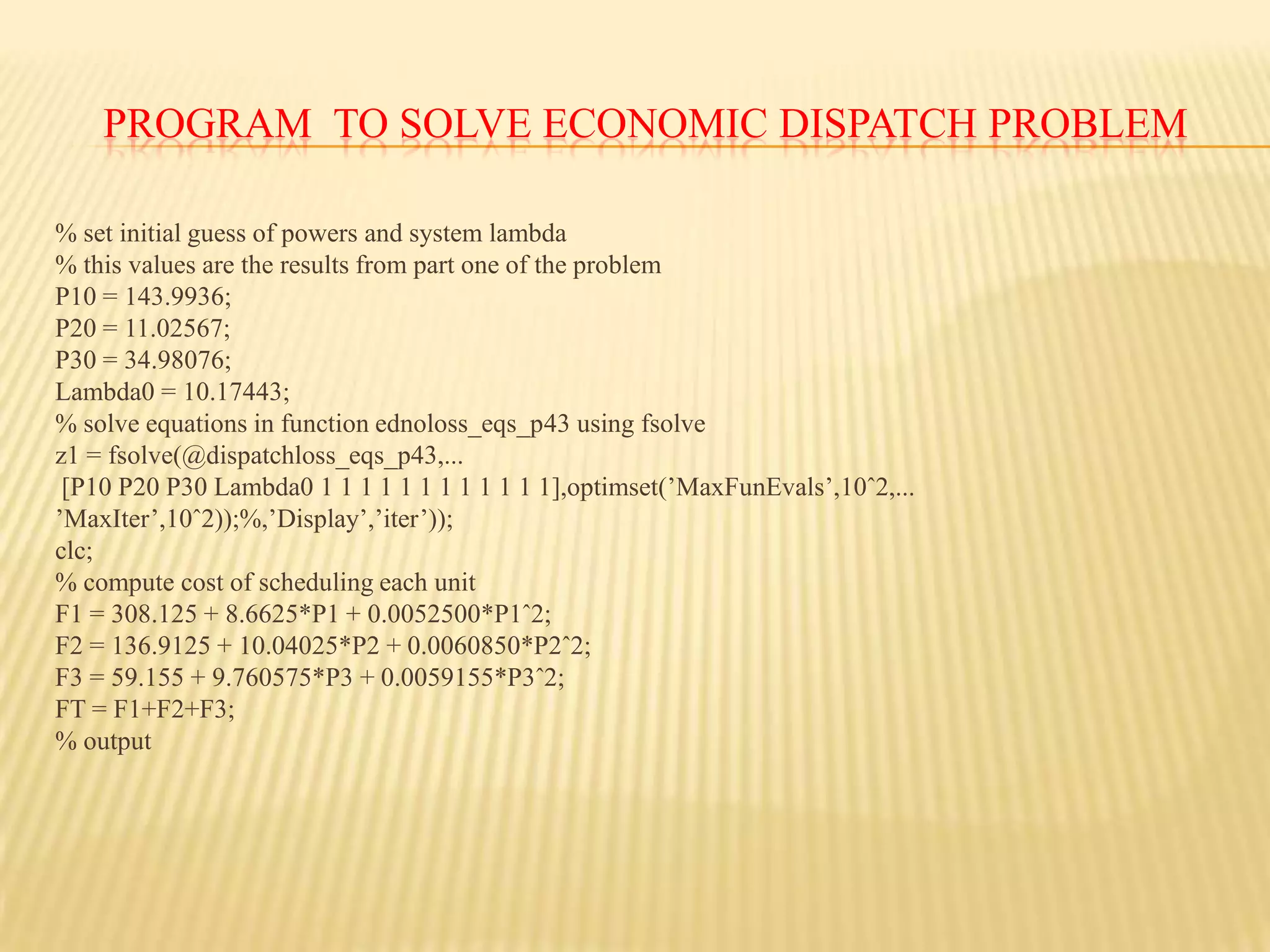
41. program to solve economic dispatch problem % set initial guess of powers and system lambda% this values are the results from part one of the problemP10 = 143.9936;P20 = 11.02567;P30 = 34.98076;Lambda0 = 10.17443;% solve equations in function ednoloss_eqs_p43 using fsolvez1 = fsolve(@dispatchloss_eqs_p43,... [P10 P20 P30 Lambda0 1 1 1 1 1 1 1 1 1 1 1 1],optimset(’MaxFunEvals’,10ˆ2,...’MaxIter’,10ˆ2));%,’Display’,’iter’));clc;% compute cost of scheduling each unitF1 = 308.125 + 8.6625*P1 + 0.0052500*P1ˆ2;F2 = 136.9125 + 10.04025*P2 + 0.0060850*P2ˆ2;F3 = 59.155 + 9.760575*P3 + 0.0059155*P3ˆ2;FT = F1+F2+F3;% output

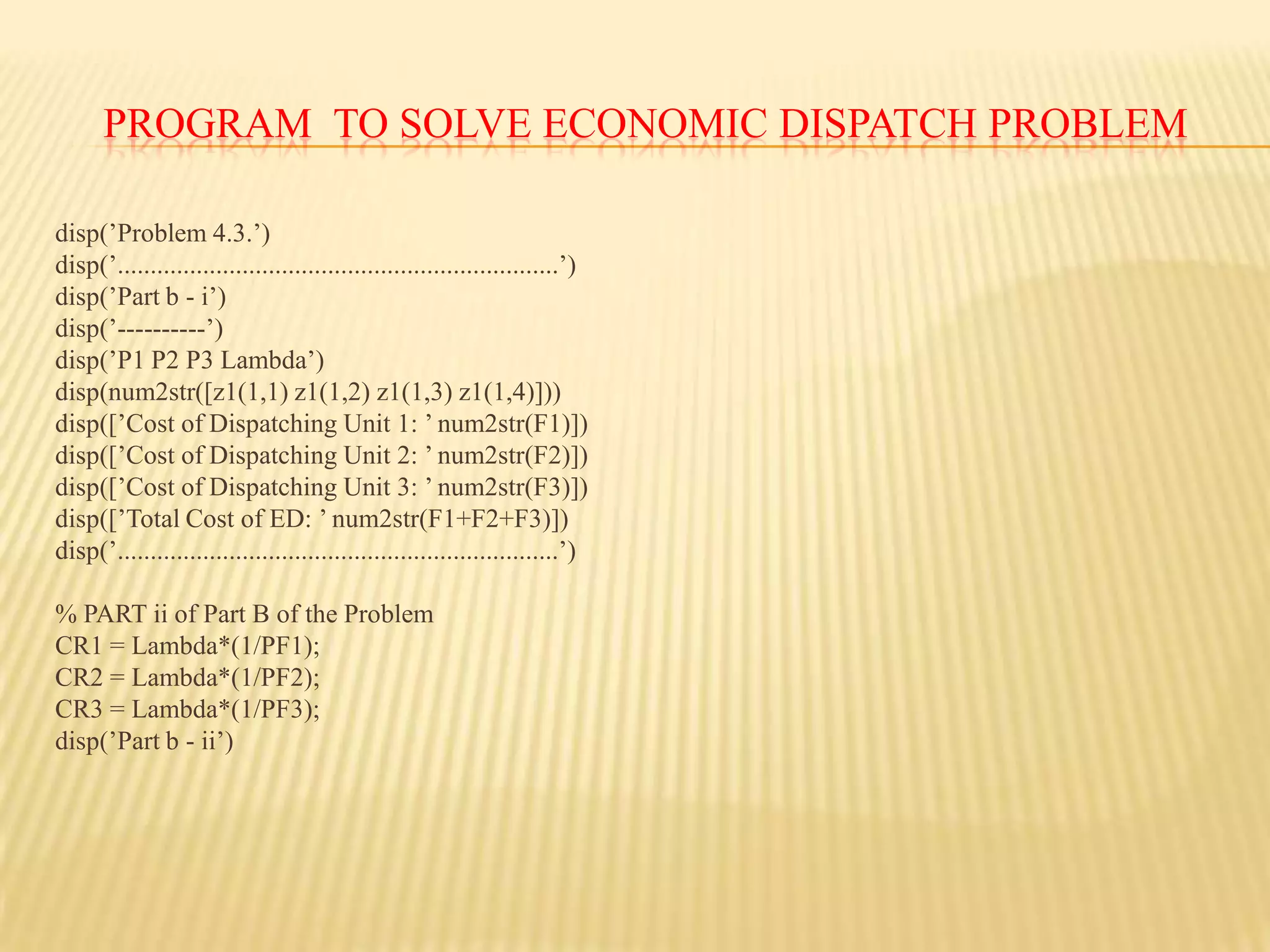
42. program to solve economic dispatch problem disp(’Problem 4.3.’)disp(’...................................................................’)disp(’Part b - i’)disp(’----------’)disp(’P1 P2 P3 Lambda’)disp(num2str([z1(1,1) z1(1,2) z1(1,3) z1(1,4)]))disp([’Cost of Dispatching Unit 1: ’ num2str(F1)])disp([’Cost of Dispatching Unit 2: ’ num2str(F2)])disp([’Cost of Dispatching Unit 3: ’ num2str(F3)])disp([’Total Cost of ED: ’ num2str(F1+F2+F3)])disp(’...................................................................’) % PART ii of Part B of the ProblemCR1 = Lambda*(1/PF1);CR2 = Lambda*(1/PF2);CR3 = Lambda*(1/PF3);disp(’Part b - ii’)

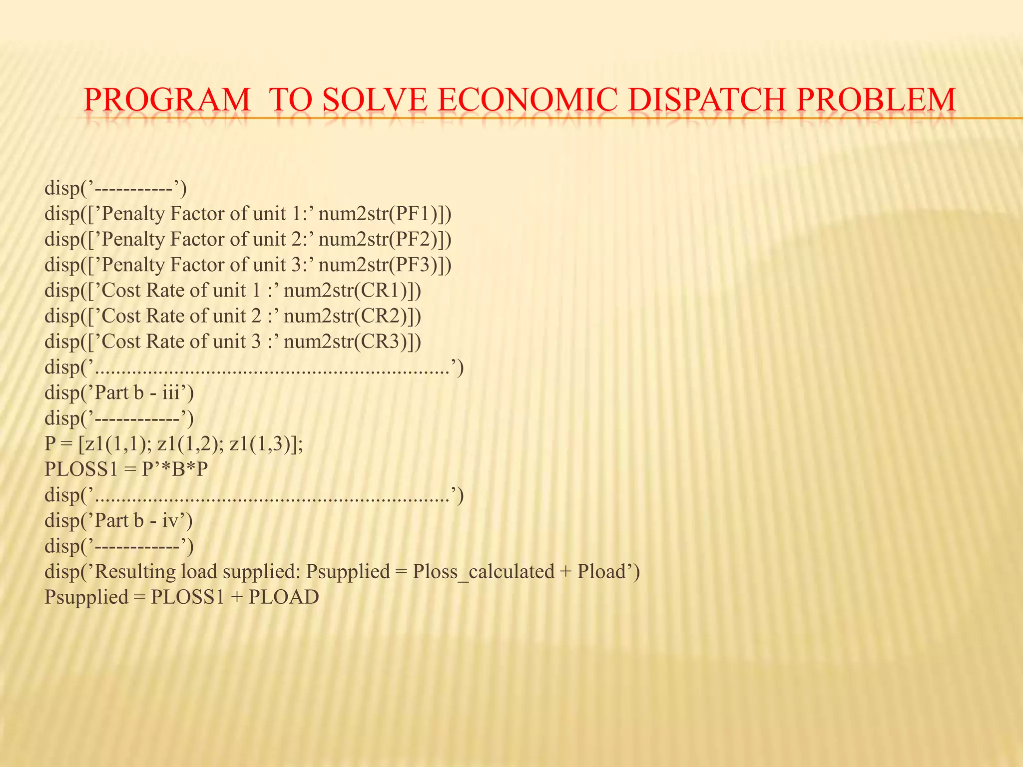
43. program to solve economic dispatch problem disp(’-----------’)disp([’Penalty Factor of unit 1:’ num2str(PF1)])disp([’Penalty Factor of unit 2:’ num2str(PF2)])disp([’Penalty Factor of unit 3:’ num2str(PF3)])disp([’Cost Rate of unit 1 :’ num2str(CR1)])disp([’Cost Rate of unit 2 :’ num2str(CR2)])disp([’Cost Rate of unit 3 :’ num2str(CR3)])disp(’...................................................................’)disp(’Part b - iii’)disp(’------------’)P = [z1(1,1); z1(1,2); z1(1,3)];PLOSS1 = P’*B*Pdisp(’...................................................................’)disp(’Part b - iv’)disp(’------------’)disp(’Resulting load supplied: Psupplied = Ploss_calculated + Pload’)Psupplied = PLOSS1 + PLOAD

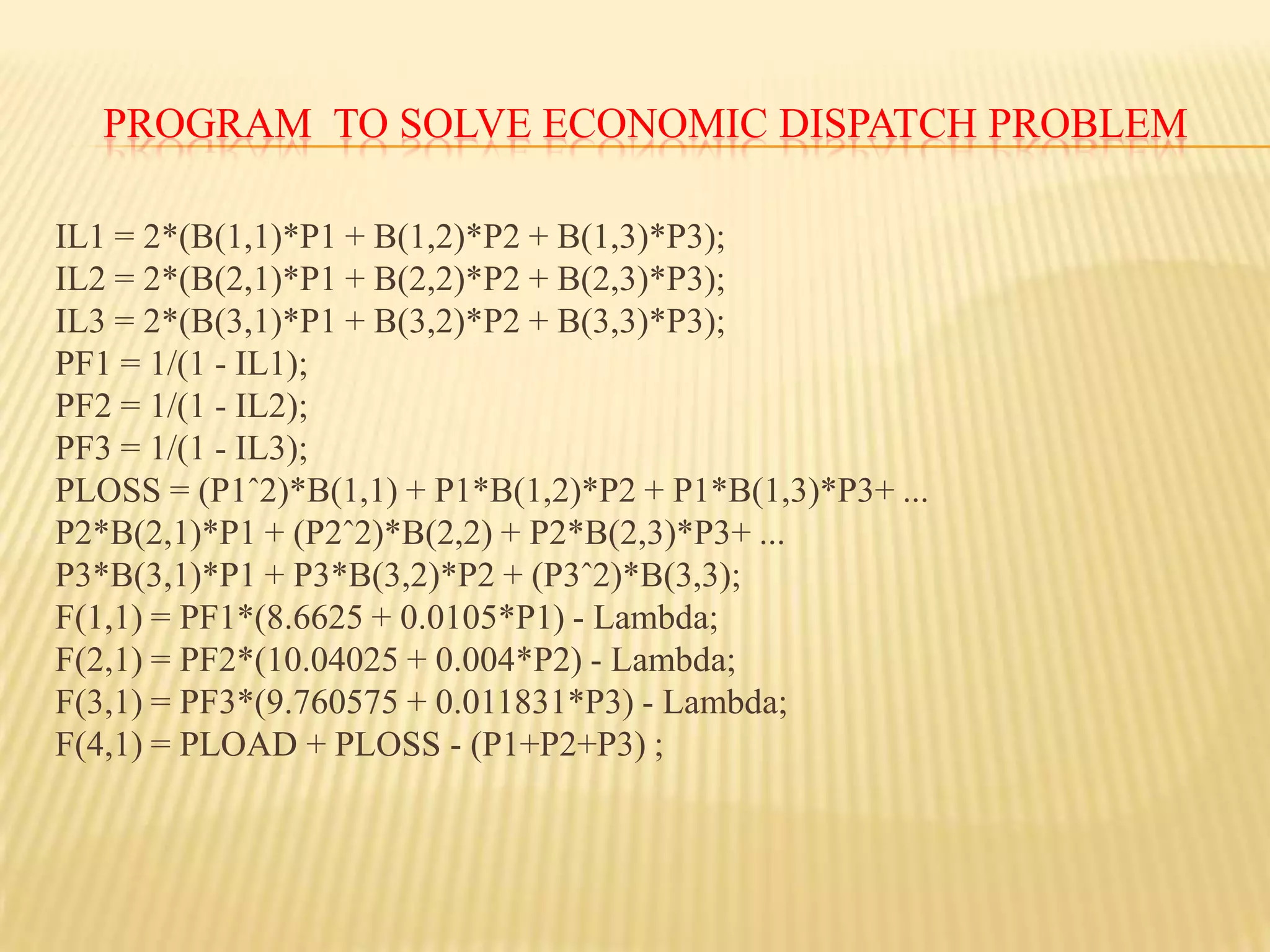
44. program to solve economic dispatch problem Function File: function F = dispatchloss_eqs_p43(z)global P1 P2 P3 Lambda IL1 IL2 IL3 PF1 PF2 PF3 PLOSS B PLOADglobal P1min P2min P3min P1max P2max P3max% Unknown variablesP1 = z(1);P2 = z(2);P3 = z(3);Lambda = z(4);IL1 = z(5);IL2 = z(6);IL3 = z(7);PF1 = z(8);PF2 = z(9);PF3 = z(10);PLOSS = z(11);% bound powers to their limitsif P3 < P3minP3 = P3min;else

45. program to solve economic dispatch problem if P3 > P3maxP3 = P3max;endendif P2 < P2minP2 = P2min;elseif P2 > P2maxP2 = P2max;endendif P1 < P1minP1 = P1min;elseif P1 > P1maxP1 = P1max;endend

46. program to solve economic dispatch problem IL1 = 2*(B(1,1)*P1 + B(1,2)*P2 + B(1,3)*P3);IL2 = 2*(B(2,1)*P1 + B(2,2)*P2 + B(2,3)*P3);IL3 = 2*(B(3,1)*P1 + B(3,2)*P2 + B(3,3)*P3);PF1 = 1/(1 - IL1);PF2 = 1/(1 - IL2);PF3 = 1/(1 - IL3);PLOSS = (P1ˆ2)*B(1,1) + P1*B(1,2)*P2 + P1*B(1,3)*P3+ ...P2*B(2,1)*P1 + (P2ˆ2)*B(2,2) + P2*B(2,3)*P3+ ...P3*B(3,1)*P1 + P3*B(3,2)*P2 + (P3ˆ2)*B(3,3);F(1,1) = PF1*(8.6625 + 0.0105*P1) - Lambda;F(2,1) = PF2*(10.04025 + 0.004*P2) - Lambda;F(3,1) = PF3*(9.760575 + 0.011831*P3) - Lambda;F(4,1) = PLOAD + PLOSS - (P1+P2+P3) ;

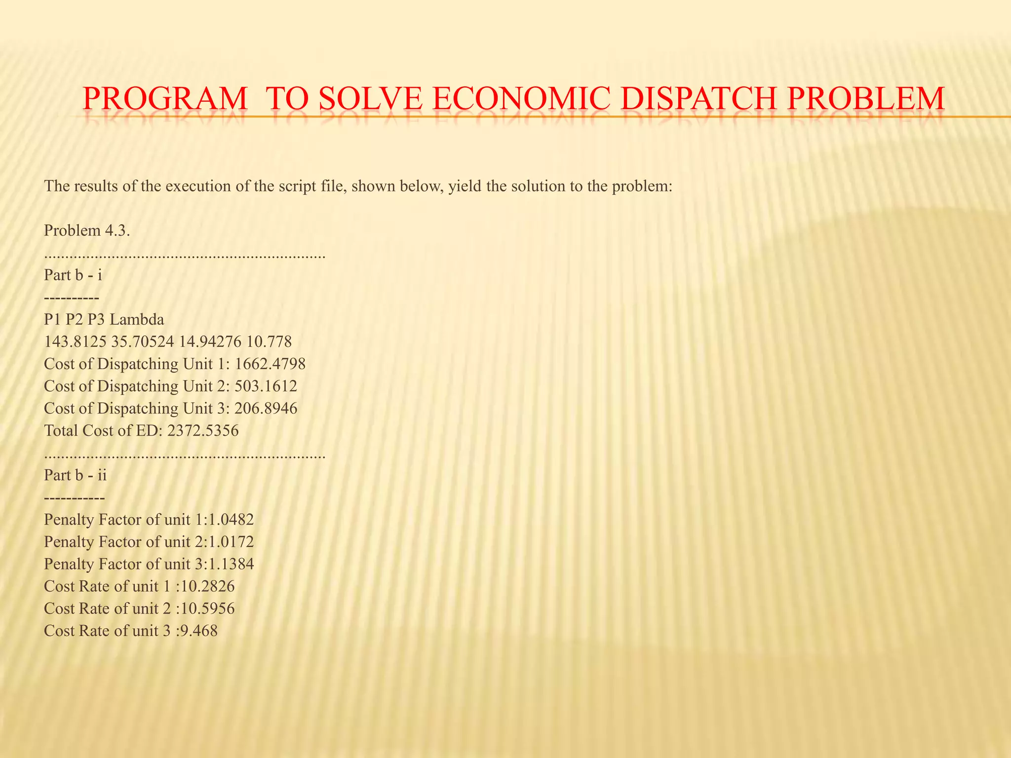
47. program to solve economic dispatch problem The results of the execution of the script file, shown below, yield the solution to the problem: Problem 4.3....................................................................Part b - i----------P1 P2 P3 Lambda143.8125 35.70524 14.94276 10.778Cost of Dispatching Unit 1: 1662.4798Cost of Dispatching Unit 2: 503.1612Cost of Dispatching Unit 3: 206.8946Total Cost of ED: 2372.5356...................................................................Part b - ii-----------Penalty Factor of unit 1:1.0482Penalty Factor of unit 2:1.0172Penalty Factor of unit 3:1.1384Cost Rate of unit 1 :10.2826Cost Rate of unit 2 :10.5956Cost Rate of unit 3 :9.468

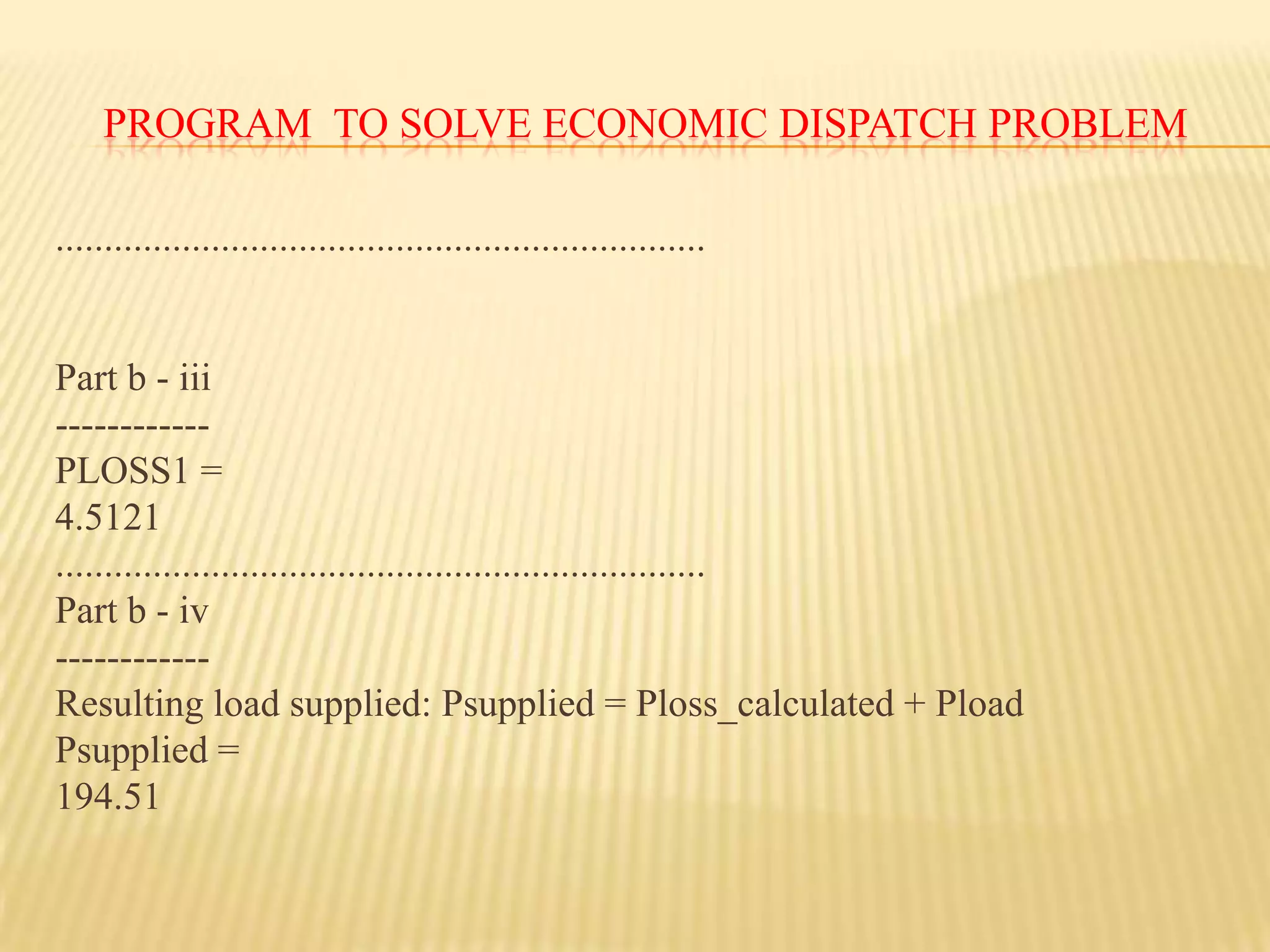
48. program to solve economic dispatch problem ................................................................... Part b - iii------------PLOSS1 =4.5121...................................................................Part b - iv------------Resulting load supplied: Psupplied = Ploss_calculated + PloadPsupplied =194.51

49. Economic Load dispatchDoes including loss formula matter? The inclusion of losses does matter; it can be seen from the results above that the consideration of losses in the scheduling changes the optimum economic dispatch, increases the total generation cost (since the total demand will now include the power dissipated in the resistive elements) and also the system lambda; the inclusion of losses it’s also a more realistic representation of what is happening in the real power system, which has losses.

50. Thank you