Topological sorting is a linear ordering of the vertices in a directed acyclic graph (DAG) where for every edge from vertex u to vertex v, u comes before v in the ordering. The algorithm uses a depth-first search approach with a stack to iteratively push and pop vertices as their adjacent vertices are explored. Breadth-first search also traverses a graph by exploring the neighbor vertices, but uses a queue rather than a stack and marks visited vertices to avoid getting stuck in cycles. The document provides pseudocode for both algorithms with an example graph to demonstrate the process.

1. BY…
M.ARCHANA
I-Msc(cs)

2. Topological sorting:
Topological sorting for Directed Acyclic Graph
(DAG) is a linear ordering of vertices such that for
every directed edge u v, vertex u comes before v in
the ordering.
 Topological Sorting for a graph is not possible if the
graph is not a DAG.
For example, a topological sorting of the following
graph is “5 4 2 3 1 0”. There can be more than one
topological sorting for a graph.

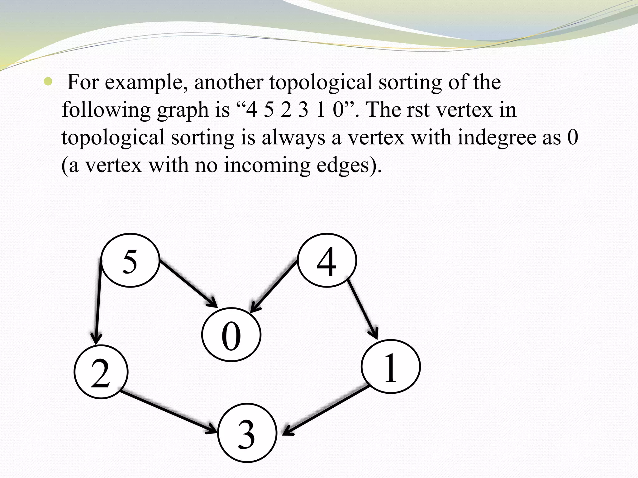
3.  For example, another topological sorting of the
following graph is “4 5 2 3 1 0”. The rst vertex in
topological sorting is always a vertex with indegree as 0
(a vertex with no incoming edges).
5 4
0
2 1
3

4. Algorithm to find topological
sorting:
We recommend to first see the implementation of DFS.
We can modify DFS to find Topological Sorting of a
graph.
 In DFS, we start from a vertex, we first print it and then
recursively call DFS for its adjacent vertices.
 In topological sorting, we use a temporary stack. We
don’t print the vertex immediately, we first recursively
call topological sorting for all its adjacent vertices, then
push it to a stack.
 Finally, print contents of the stack. Note that a vertex is
pushed to stack only when all of its adjacent vertices (and
their adjacent vertices and so on) are already in the stack.

5. Breadth first traversal:
 Breadth First Search (BFS) algorithm traverses a
graph in a breadthward motion and uses a queue to
remember to get the next vertex to start a search,
when a dead end occurs in any iteration.
 Breadth First Traversal (or Search) for a graph is similar to
Breadth First Traversal of a tree (See method 2 of this
post).
 The only catch here is, unlike trees, graphs may contain
cycles, so we may come to the same node again.

6. Cont.,
 To avoid processing a node more than once, we use a
Boolean visited array.
 For simplicity, it is assumed that all vertices are reachable
from the starting vertex.
 For example, in the following graph, we start traversal
from vertex 2.
 When we come to vertex 0, we look for all adjacent
vertices of it.
 2 is also an adjacent vertex of 0.
 If we don’t mark visited vertices, then 2 will be
processed again and it will become a non-terminating
process.

7. A Breadth First Traversal of the following graph is 2, 0,
3, 1.
start
0 1
2 3

8. Example:

9. cont.,
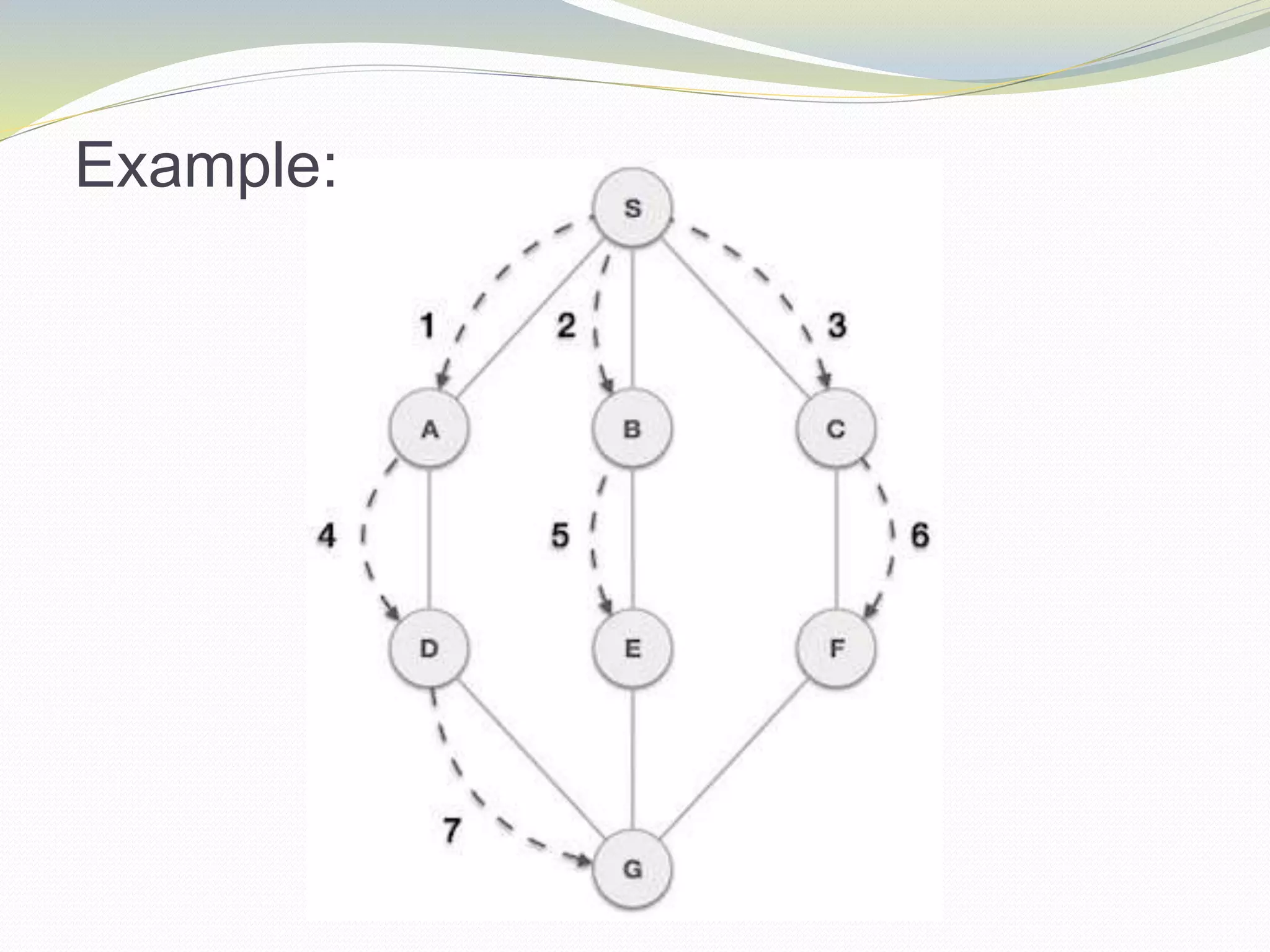
 As in the example given above, BFS algorithm traverses from
A to B to E to F first then to C and G lastly to D. It employs the
following rules. lastly to D. It employs the following rules.
 Rule 1 − Visit the adjacent unvisited vertex. Mark it as visited.
Display it. Insert it in a − Visit the adjacent unvisited vertex.
Mark it as visited. Display it. Insert it in a queue. queue. Rule
 Rule 2 − If no adjacent vertex is found, remove the first vertex
from the queue. − If no adjacent vertex is found, remove the
first vertex from the queue.
 Rule 3 − Repeat Rule 1 and Rule 2 until the queue is empty.

10. Step 1:
Initialize the
queue.

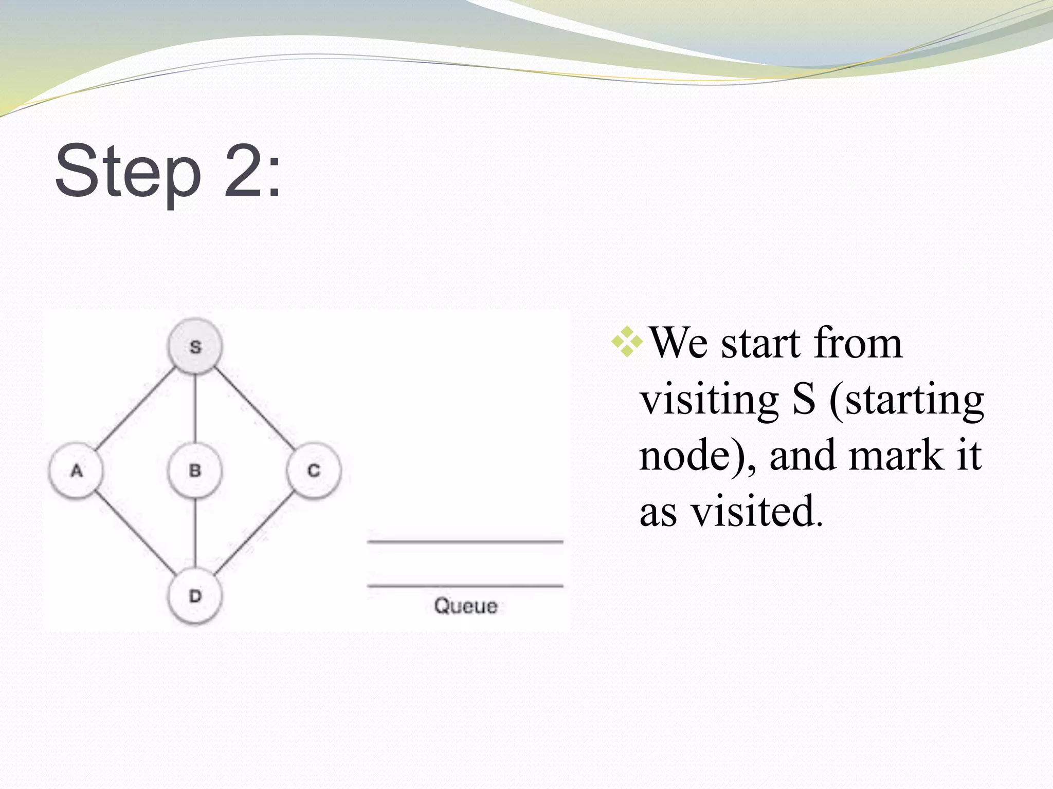
11. Step 2:
We start from
visiting S (starting
node), and mark it
as visited.

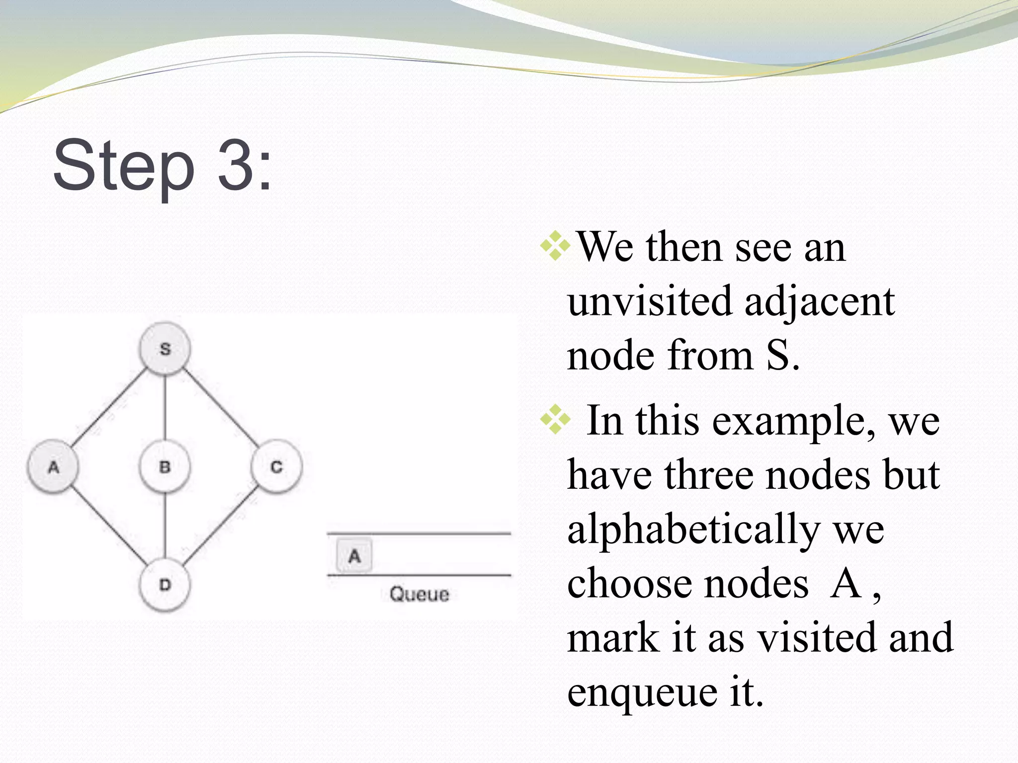
12. Step 3:
We then see an
unvisited adjacent
node from S.
 In this example, we
have three nodes but
alphabetically we
choose nodes A ,
mark it as visited and
enqueue it.

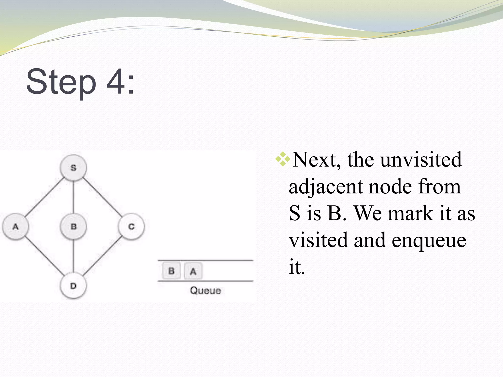
13. Step 4:
Next, the unvisited
adjacent node from
S is B. We mark it as
visited and enqueue
it.

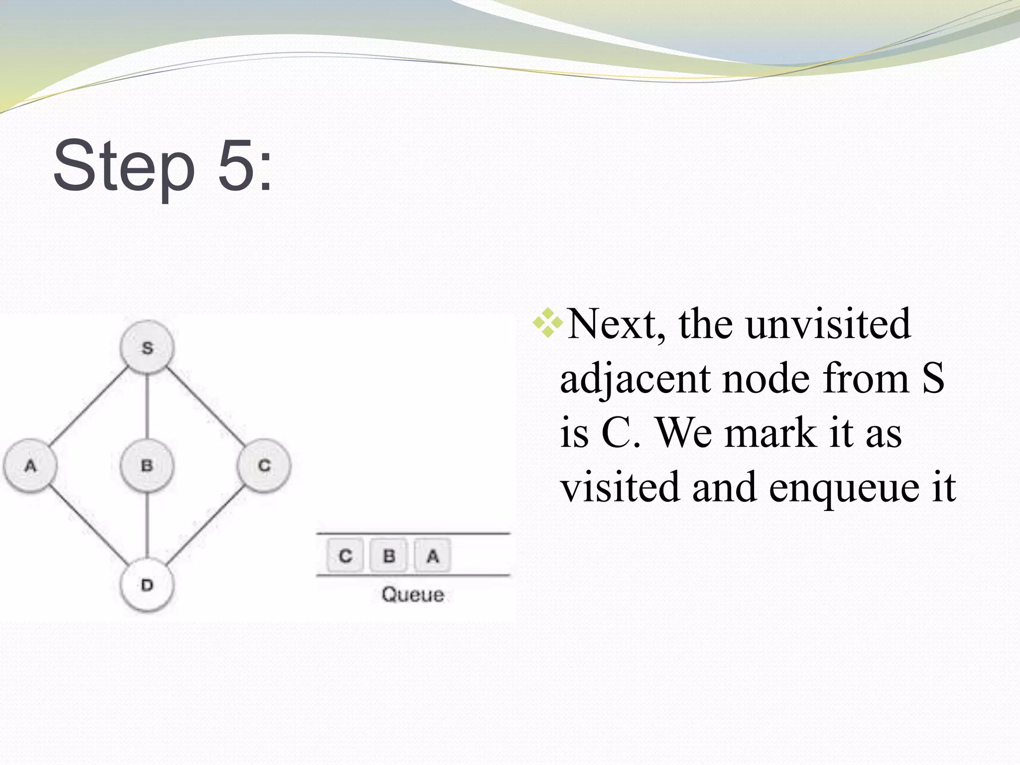
14. Step 5:
Next, the unvisited
adjacent node from S
is C. We mark it as
visited and enqueue it

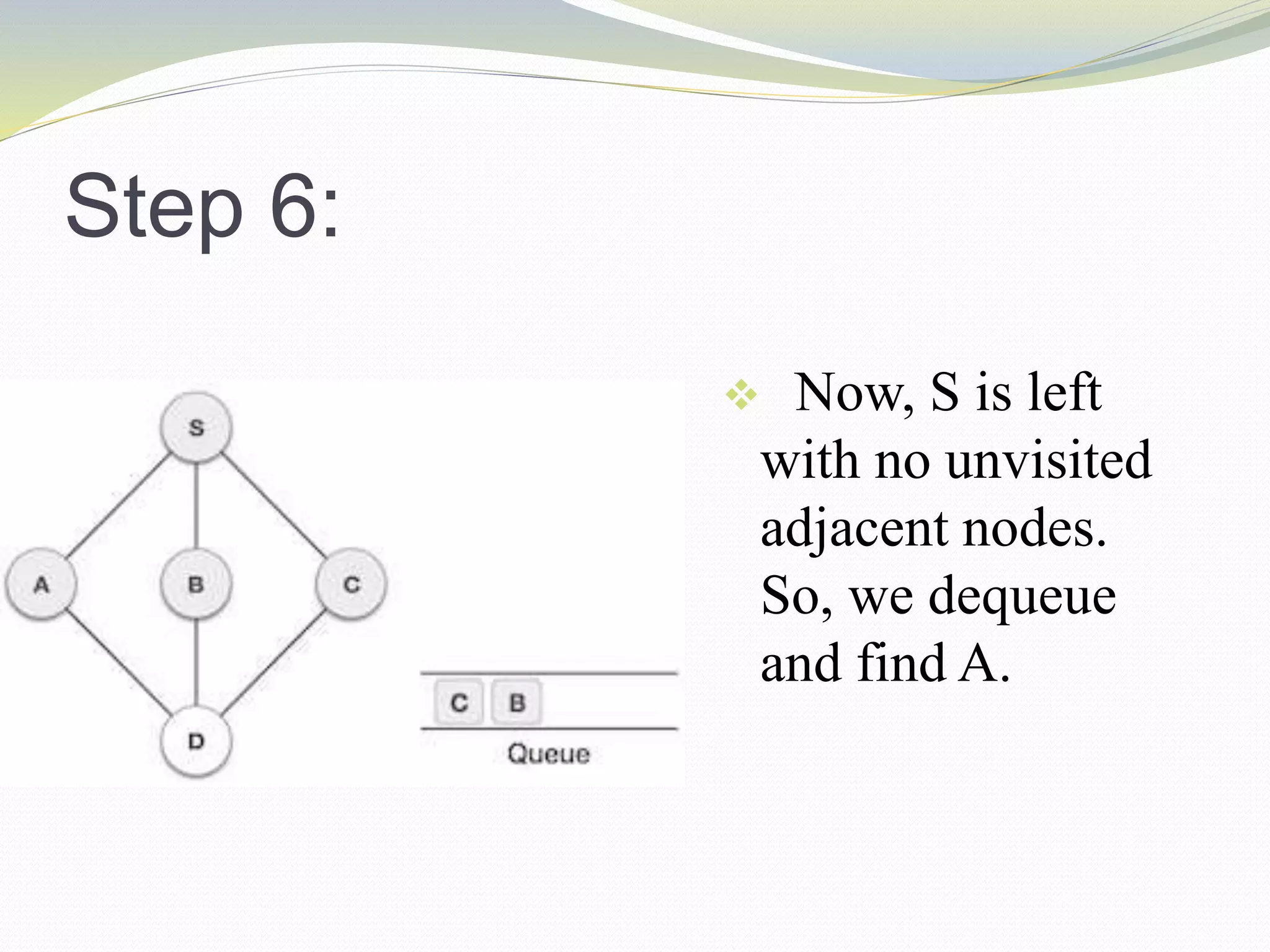
15. Step 6:
 Now, S is left
with no unvisited
adjacent nodes.
So, we dequeue
and find A.

16. Step 7:
From A we have
D as unvisited
adjacent node. We
mark it as visited
and enqueue it