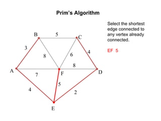
The document provides an introduction to graph theory, explaining the fundamental concepts such as vertices, edges, and different types of graphs including directed, undirected, and weighted graphs. It discusses graph properties like connectivity, paths, cycles, traversal methods (BFS and DFS), and algorithms for operations like minimum spanning trees using Kruskal's and Prim's algorithms. Additionally, it illustrates real-life applications of graphs and introduces techniques for graph representation and traversal.


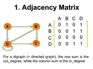
![Adjacency Matrix
• Assume V = {1, 2, …, n}
• An adjacency matrix represents the graph as a
n x n matrix A:
– A[i, j] = 1 if edge (i, j) ∈ E (or weight of edge)
= 0 if edge (i, j) ∉ E
– Storage requirements: O(V2
)
• A dense representation](https://image.slidesharecdn.com/graphs-190327145219/85/Graphs-16-320.jpg)


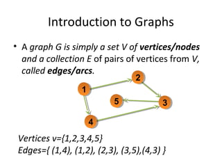
![#include<stdio.h>
int a[20][20],q[20],visited[20],n,f=-1,r=-1;
void bfs(int v)
{
int i;
for (i=0;i<n;i++) // check all the vertices in the graph
{
if(a[v][i] != 0 && visited[i] == 0) // adjacent to v and not visited
{
r=r+1;
q[r]=i; // insert them into queue
visited[i]=1; // mark the vertex visited
printf("%d ",i);
}
}
f=f+1; // remove the vertex at front of the queue
if(f<=r) // as long as there are elements in the queue
bfs(q[f]); // peform bfs again on the vertex at front of the queue
}
Entire program is at below link
http://enthusiaststudent.blogspot.com/2019/03/breadth-first-search-c-program.html
BFS Program](https://image.slidesharecdn.com/graphs-190327145219/85/Graphs-23-320.jpg)


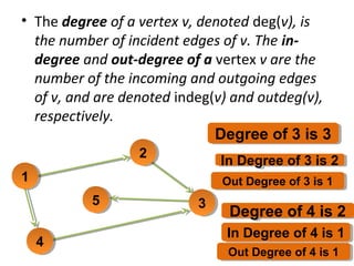
![#include<stdio.h>
int a[20][20],q[20],visited[20],n;
void dfs(int v)
{
int i;
for (i=0;i<n;i++) // check all the vertices in the graph
{
if(a[v][i] != 0 && visited[i] == 0) // adjacent to v and not visited
{
visited[i]=1; // mark the vertex visited
printf("%d ",i);
dfs(i);
}
}
}
Entire program is at below link
http://enthusiaststudent.blogspot.com/2019/03/depth-first-search-c-program.html
DFS Program](https://image.slidesharecdn.com/graphs-190327145219/85/Graphs-31-320.jpg)