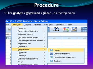
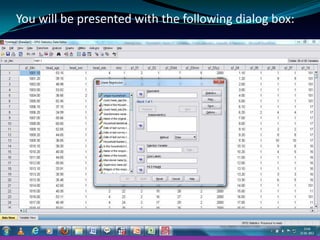
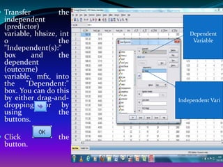
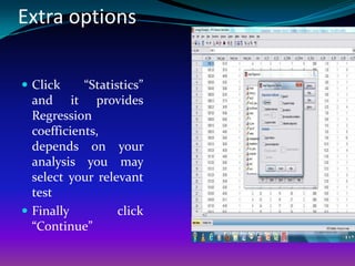
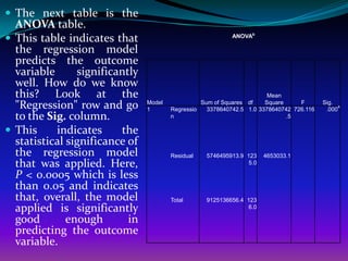
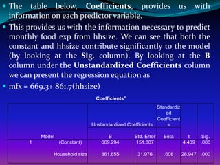
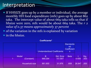
Srinivasulu Rajendran
 Centre for the Study of Regional Development (CSRD)


Jawaharlal Nehru University (JNU)
                      New Delhi
                        India
              r.srinivasulu@gmail.com
Objective of the session


        To understand How
       HHsize influences the
        monthly per capita
      total expenditure of the
      households based OLS
1. What is the procedure to
perform Regression?
2. How do we interpret results?
4. What are procedure available
for estimating poverty line and
Poverty rate and how to do with
Econometric software
Identify the relationship between variables that
we want to perform Scatter plot for outliers and
type of relationship


 Monthly HH food Expenditure and HHSIZE
Linear Regression Analysis using
             SPSS
Objectives
 Regression analysis is    the next step up after
 correlation; it is used when we want to predict the
 value of a variable based on the value of another
 variable. In this case, the variable we are using to
 predict the other variable's value is called the
 independent variable or sometimes the predictor
 variable. The variable we are wishing to predict is
 called the dependent variable or sometimes the
 outcome variable.
Assumption
 Variables are approximately normally distributed
  (see Testing for Normality guide).
 There is a linear relationship between the two
  variables.
 There are classical assumption ……..
Step 1
Procedure
1.Click Analyze > Regression > Linear... on the top menu.
You will be presented with the following dialog box:
Step 2
 Transfer         the
  independent
  (predictor)
  variable, hhsize, int       Dependent
  o                 the        Variable
  "Independent(s):"
  box      and      the
  dependent
  (outcome)
  variable, mfx, into
  the "Dependent:"
  box. You can do this
  by either drag-and-     Independent Vari
  dropping or by
  using             the
  buttons.

 Click            the
  button.
Step 2
Extra options

 Click     “Statistics”
  and it provides
  Regression
  coefficients,
  depends on your
  analysis you may
  select your relevant
  test
 Finally          click
  “Continue”
Plot - Options

 Click “Plot” and it
  provides option to
  plot      histogram,
  normal probability,
  etc, depends on
  your analysis you
  may select your
  relevant plot
 Finally         click
  “Continue”
Click    “OK”
 to get results
 in the output
 viewer
Output of Linear Regression
         Analysis
 SPSS will generate quite a
  few tables in its results
  section     for   a     linear
  regression.
 In this session, we are going
  to look at the important                          Model Summary
  tables Model Summary
  table.
 This table provides the R
  and R2 value. The R value is
  0.608, which represents the
                                                              Adjusted R Std. Error of
  simple            correlation    Model   R        R Square   Square     the Estimate
                                                a
  and, therefore, indicates a      1       .608          .370        .370      2157.08
  high degree of correlation.
  The R2 value indicates how
  much of the dependent
  variable, monthly HH food
  exp, can be explained by the
  independent
  variable, hhsize. In this
  case,     37.0%    can      be
  explained.
 The next table is the
  ANOVA table.
 This table indicates that                                 ANOVAb

  the regression model
  predicts the outcome
  variable      significantly
  well. How do we know
  this? Look at the                                                     Mean
  "Regression" row and go       Model
                                1       Regressio
                                                  Sum of Squares df    Square     F
                                                    3378640742.5 1.0 3378640742 726.116
                                                                                          Sig.
                                                                                           .000
                                                                                                a


  to the Sig. column.                   n                                     .5

 This     indicates     the
  statistical significance of
  the regression model                  Residual   5746495913.9 123    4653033.1
  that was applied. Here,                                        5.0

  P < 0.0005 which is less
  than 0.05 and indicates
  that, overall, the model              Total      9125136656.4 123
  applied is significantly                                       6.0

  good        enough       in
  predicting the outcome
  variable.
 The   table below, Coefficients, provides us with
  information on each predictor variable.
 This provides us with the information necessary to predict
  monthly food exp from hhsize. We can see that both the
  constant and hhsize contribute significantly to the model
  (by looking at the Sig. column). By looking at the B
  column under the Unstandardized Coefficients column
  we can present the regression equation as
 mfx = 669.3+ 861.7(hhsize)
                                  Coefficientsa
                                                             Standardiz
                                                                 ed
                                                             Coefficient
                                 Unstandardized Coefficients      s

            Model                       B          Std. Error   Beta         t     Sig.
        1           (Constant)       669.294       151.807                 4.409   .000

                Household size       861.655         31.976     .608       26.947 .000
Interpretation
 If HHSIZE goes up by a member or individual, the average
  monthly HH food expenditure (mfx) goes up by about 862
  taka. The intercept value of about 669 taka tells us that if
  hhsize were zero, mfx would be about 669 taka. The r 2
  value of 0.37 means approximately 37 percent
 of the variation in the mfx is explained by variation
 in the hhsize.
                                Coefficientsa
                                                           Standardiz
                                                               ed
                                                           Coefficient
                               Unstandardized Coefficients      s

          Model                       B          Std. Error   Beta         t     Sig.
      1           (Constant)       669.294       151.807                 4.409   .000

              Household size       861.655         31.976     .608       26.947 .000

Topic17 regression spss

  • 1.
    Srinivasulu Rajendran Centrefor the Study of Regional Development (CSRD) Jawaharlal Nehru University (JNU) New Delhi India r.srinivasulu@gmail.com
  • 2.
    Objective of thesession To understand How HHsize influences the monthly per capita total expenditure of the households based OLS
  • 3.
    1. What isthe procedure to perform Regression? 2. How do we interpret results? 4. What are procedure available for estimating poverty line and Poverty rate and how to do with Econometric software
  • 4.
    Identify the relationshipbetween variables that we want to perform Scatter plot for outliers and type of relationship  Monthly HH food Expenditure and HHSIZE
  • 5.
  • 6.
    Objectives  Regression analysisis the next step up after correlation; it is used when we want to predict the value of a variable based on the value of another variable. In this case, the variable we are using to predict the other variable's value is called the independent variable or sometimes the predictor variable. The variable we are wishing to predict is called the dependent variable or sometimes the outcome variable.
  • 7.
    Assumption  Variables areapproximately normally distributed (see Testing for Normality guide).  There is a linear relationship between the two variables.  There are classical assumption ……..
  • 8.
  • 9.
    Procedure 1.Click Analyze >Regression > Linear... on the top menu.
  • 10.
    You will bepresented with the following dialog box:
  • 11.
  • 12.
     Transfer the independent (predictor) variable, hhsize, int Dependent o the Variable "Independent(s):" box and the dependent (outcome) variable, mfx, into the "Dependent:" box. You can do this by either drag-and- Independent Vari dropping or by using the buttons.  Click the button.
  • 13.
  • 14.
    Extra options  Click “Statistics” and it provides Regression coefficients, depends on your analysis you may select your relevant test  Finally click “Continue”
  • 15.
    Plot - Options Click “Plot” and it provides option to plot histogram, normal probability, etc, depends on your analysis you may select your relevant plot  Finally click “Continue”
  • 16.
    Click “OK” to get results in the output viewer
  • 17.
    Output of LinearRegression Analysis
  • 18.
     SPSS willgenerate quite a few tables in its results section for a linear regression.  In this session, we are going to look at the important Model Summary tables Model Summary table.  This table provides the R and R2 value. The R value is 0.608, which represents the Adjusted R Std. Error of simple correlation Model R R Square Square the Estimate a and, therefore, indicates a 1 .608 .370 .370 2157.08 high degree of correlation. The R2 value indicates how much of the dependent variable, monthly HH food exp, can be explained by the independent variable, hhsize. In this case, 37.0% can be explained.
  • 19.
     The nexttable is the ANOVA table.  This table indicates that ANOVAb the regression model predicts the outcome variable significantly well. How do we know this? Look at the Mean "Regression" row and go Model 1 Regressio Sum of Squares df Square F 3378640742.5 1.0 3378640742 726.116 Sig. .000 a to the Sig. column. n .5  This indicates the statistical significance of the regression model Residual 5746495913.9 123 4653033.1 that was applied. Here, 5.0 P < 0.0005 which is less than 0.05 and indicates that, overall, the model Total 9125136656.4 123 applied is significantly 6.0 good enough in predicting the outcome variable.
  • 20.
     The table below, Coefficients, provides us with information on each predictor variable.  This provides us with the information necessary to predict monthly food exp from hhsize. We can see that both the constant and hhsize contribute significantly to the model (by looking at the Sig. column). By looking at the B column under the Unstandardized Coefficients column we can present the regression equation as  mfx = 669.3+ 861.7(hhsize) Coefficientsa Standardiz ed Coefficient Unstandardized Coefficients s Model B Std. Error Beta t Sig. 1 (Constant) 669.294 151.807 4.409 .000 Household size 861.655 31.976 .608 26.947 .000
  • 21.
    Interpretation  If HHSIZEgoes up by a member or individual, the average monthly HH food expenditure (mfx) goes up by about 862 taka. The intercept value of about 669 taka tells us that if hhsize were zero, mfx would be about 669 taka. The r 2 value of 0.37 means approximately 37 percent  of the variation in the mfx is explained by variation  in the hhsize. Coefficientsa Standardiz ed Coefficient Unstandardized Coefficients s Model B Std. Error Beta t Sig. 1 (Constant) 669.294 151.807 4.409 .000 Household size 861.655 31.976 .608 26.947 .000