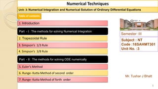
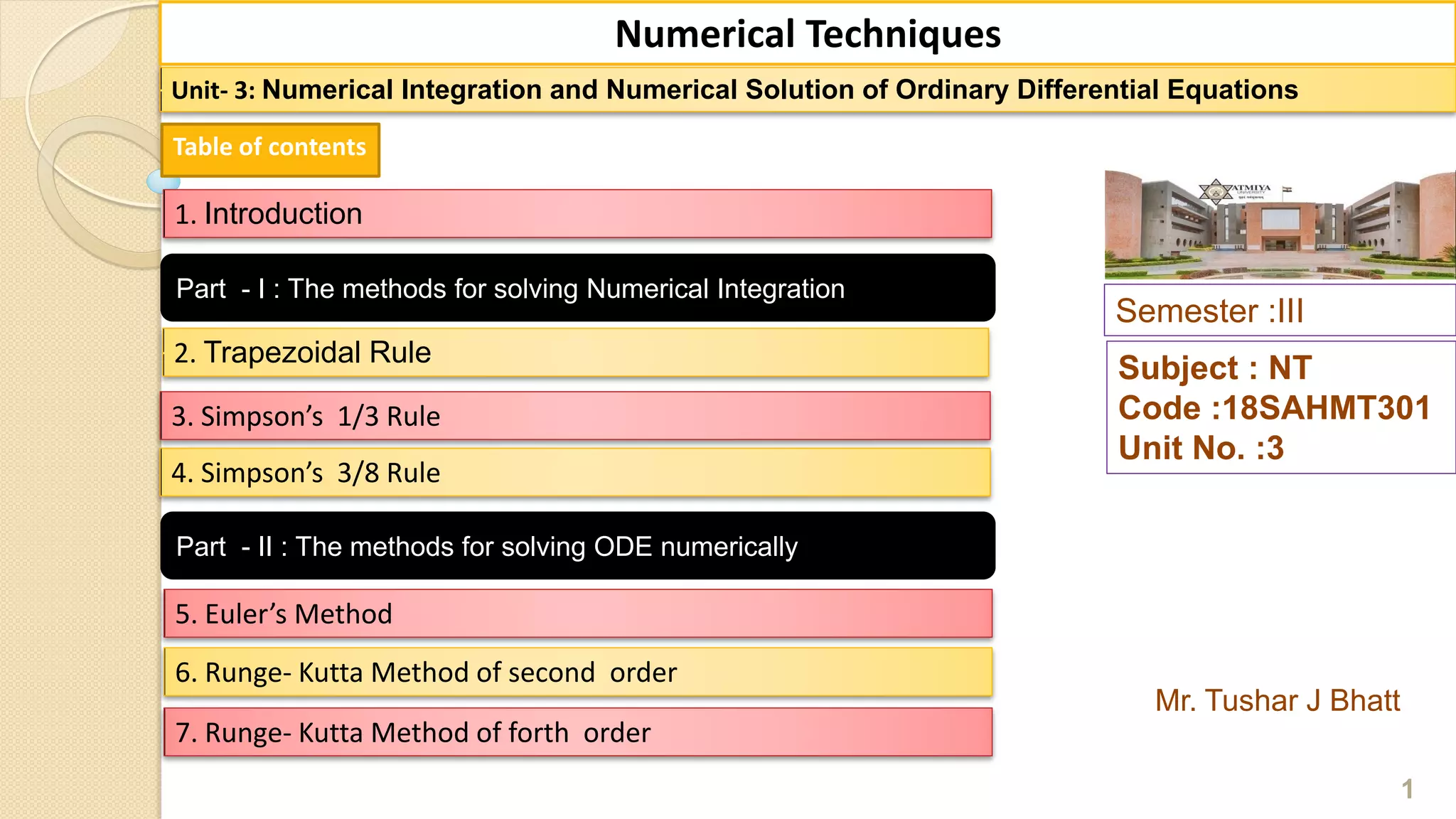
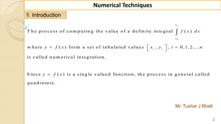
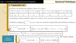
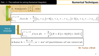
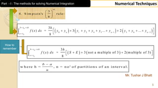
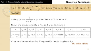
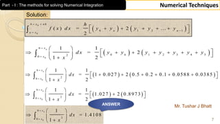
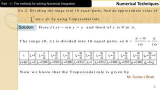
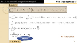
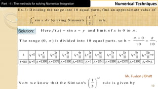
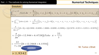
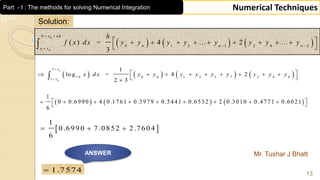
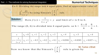
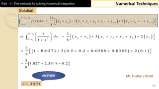
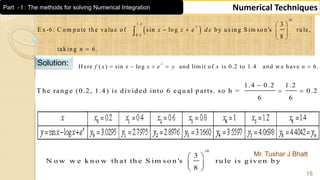
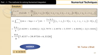
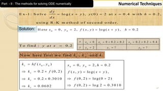
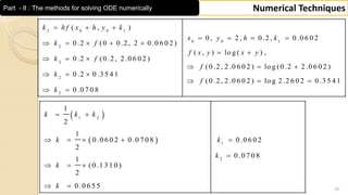
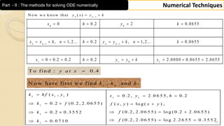
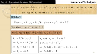
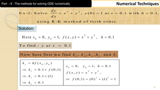
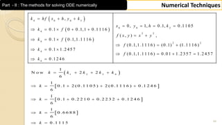
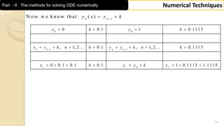
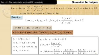
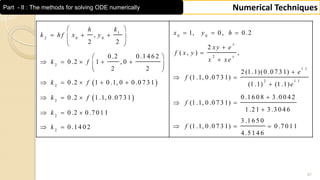
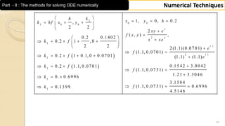
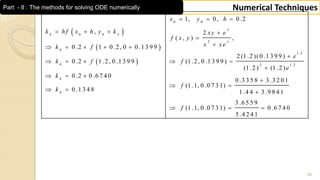
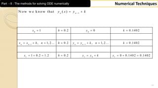
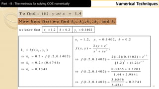
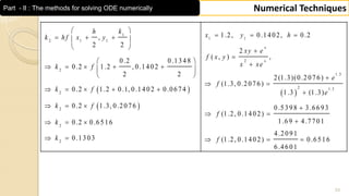
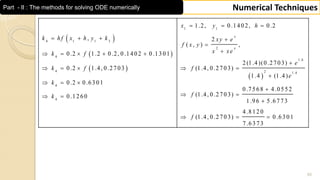
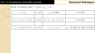
Semester :III
Mr. Tushar J Bhatt
Subject : NT
Code :18SAHMT301
Unit No. :3
1
Numerical Techniques
Unit- 3: Numerical Integration and Numerical Solution of Ordinary Differential Equations
1. Introduction
Table of contents
5. Euler’s Method
6. Runge- Kutta Method of second order
7. Runge- Kutta Method of forth order
2. Trapezoidal Rule
3. Simpson’s 1/3 Rule
4. Simpson’s 3/8 Rule
Part - I : The methods for solving Numerical Integration
Part - II : The methods for solving ODE numerically
Mr. Tushar J Bhatt
2
Numerical Techniques
1. Introduction
0
T h e p ro c e ss o f c o m p u tin g th e v a lu e o f a d e fin ite in te g ra l ( )
w h e re ( ) fo rm a se t o f ta b u la te d v a lu e s , , 0 ,1, 2 , ...
is c a lle d n u m e ric a l in te g ra tio n .
S in c e ( ) is a sin g le v a lu e d
nx
x
i i
f x d x
y f x x y i n
y f x
  
 


fu n c tio n , th e p ro c e ss in g e n e ra l c a lle d
q u a d ra tu re .
Mr. Tushar J Bhatt
3
Numerical Techniques
2. Trapezoidal rule
0 1 0 2 0 1 0 0
0 1 2 1
C o n sid er th e fo llo w in g tab u lar valu es o f x an d y :
2 .... ( 1)
.
....
A cco rd in g to ab o ve tab u lar valu es o f x a n d y, if w e w an t to calcu late th e valu es
o f
n n
n n
x x a x x h x x h x x n h x x n h b
y y y y y y


          
0
0
d efin ite in teg ral ( ) th en w e u sed th e trap ezo id al ru le d efin ed as fo llo w s:
b x n h
a x
f x d x
 

   
0
0
0 1 2 1
( ) = 2 ...
2
b x n h
n n
a x
h
f x d x y y y y y
 


     
 
   
0
0
( ) = 2
2
b x n h
a x
h
f x d x S E R
 

   
How to
remember
w h e r e h = , n = n o ' o f p a r t i t i o n s o f a n i n t e r v a l.
b a
n

Part - I : The methods for solving Numerical Integration
Mr. Tushar J Bhatt
4
Numerical Techniques
1
3 . S im p s o n 's ru le :
3
r d
 
 
 
   
0
0
( ) = 4 2 ( )
3
b x n h
a x
h
f x d x S E O E
 

    
How to
remember
     
0
0
0 1 3 1 2 4 2
( ) = 4 ... 2 ...
3
b x nh
n n n
a x
h
f x dx y y y y y y y y
 
 

         
 
w h e re h = , n = n o ' o f p a rtitio n s o f a n i n te rv a l.
b a
n

Part - I : The methods for solving Numerical Integration
Mr. Tushar J Bhatt
5
Numerical Techniques
3
4 . S im p s o n 's ru le :
8
th
 
 
 
   
0
0
3
( ) = 3 not a m ultiple of 3 2(m ultiple of 3)
8
b x nh
a x
h
f x dx S E
 

    
How to
remember
     
0
0
0 1 2 4 5 1 3 6 3
3
( ) = 3 ... 2 ...
8
b x nh
n n n
a x
h
f x dx y y y y y y y y y y
 
 

          
 
w h e re h = , n = n o ' o f p a rtitio n s o f a n i n te rv a l.
b a
n

Part - I : The methods for solving Numerical Integration
Mr. Tushar J Bhatt
6
Numerical Techniques
6
20
E x -1 : E valu ate b y u sin g T rap ezo id al ru le tak in g 1 .
1
d x
h
x



Solution:
2
1
H e re ( ) a n d lim it o f is 0 to 6 .
1
f x y x
x
 

N o w w e m ak e a tab le o f x an d y as fo llo w s :
0 1 2 3 4 5 6
0 1 2 3 4 5 62
0 1 2 3 4 5 6
1
1 0.5 0.2 0.1 0.0588 0.0385 0.027
1
n
x x x x x x x x
y y y y y y y y y
x
      
        

N o w w e k n o w th at th e T rap ezo id al ru le is g iven b y
Part - I : The methods for solving Numerical Integration
Mr. Tushar J Bhatt
7
Numerical Techniques
Solution:
   
0
0
0 1 2 1
( ) = 2 ...
2
b x n h
n n
a x
h
f x d x y y y y y
 


     
 
   0
6
0 6 1 2 3 4 520
1 1
= 2
21
nx
x
d x y y y y y y y
x


 
           

   
0
6
20
1 1
= 1 0.027 2 0.5 0.2 0.1 0.0588 0.0385
21
nx
x
dx
x


 
          
 

   
0
6
20
1 1
= 1.027 2 0.8973
21
nx
x
dx
x


 
     
 

0
6
20
1
= 1.4108
1
nx
x
dx
x


 
  
 

ANSWER
Part - I : The methods for solving Numerical Integration
Mr. Tushar J Bhatt
8
Numerical Techniques
0
E x -2 : D ivid in g th e ran g e in to 1 0 eq u al p arts, fin d an ap p ro x im ate valu e o f
sin b y u sin g T rap ezo id al ru le.x d x


Solution: H ere ( ) sin an d lim it o f is 0 to .f x x y x  
0
T h e ran g e (0 , ) is d ivid ed in to 1 0 eq u al p arts. so h = .
1 0 1 0
 



N o w w e k n o w th at th e T rap ezo id al ru le is g iven b y
Part - I : The methods for solving Numerical Integration
Mr. Tushar J Bhatt
9
Numerical Techniques
Solution:
   
0
0
0 1 2 1
( ) = 2 ...
2
b x n h
n n
a x
h
f x d x y y y y y
 


     
 
     0
0 10 1 2 3 4 5 6 7 8 9
0
sin = 2
10 2
nx
x
x dx y y y y y y y y y y y
 

           
 

   0 0 2 0.3090 0.5878 0.8090 0.9511 1.0000 0.9511 0.8090 0.5878 0.3090
10 2

            

 
22
0 12.6276 ( )
20 7
T ake

  
1.9843
ANSWER
 
2 2
0 12.6276
7 20
 

Part - I : The methods for solving Numerical Integration
Mr. Tushar J Bhatt
10
Numerical Techniques
0
E x -3 : D ivid in g th e ran g e in to 1 0 eq u al p arts, fin d an ap p ro x im ate valu e o f
1
sin b y u sin g S im so n 's ru le.
3
rd
x d x
  
 
 

Solution: H ere ( ) sin an d lim it o f is 0 to .f x x y x  
0
T h e ran g e (0 , ) is d ivid ed in to 1 0 eq u al p arts. so h = .
1 0 1 0
 



1
N o w w e k n o w th a t th e S im so n 's ru le is g iv e n b y
3
r d
 
 
 
Part - I : The methods for solving Numerical Integration
Mr. Tushar J Bhatt
11
Numerical Techniques
Solution:
       0
0 10 1 3 5 7 9 2 4 6 8
0
sin = 4 2
1 0 3
nx
x
x d x y y y y y y y y y y y
 

           
 

     0 0 4 0.3090 0.8090 1.0000 0.8090 0.3090 2 0.5878 0.9511 0.9511 0.5878
10 3

            

 
22
0 12.944 6.4720 ( )
30 7
T ake

   
1.9342
ANSWER
     
0
0
0 1 3 1 2 4 2
( ) = 4 ... 2 ...
3
b x nh
n n n
a x
h
f x dx y y y y y y y y
 
 

         
 
 
22
0 12.3068 6.1556
7 30
  

Part - I : The methods for solving Numerical Integration
Mr. Tushar J Bhatt
12
Numerical Techniques
5
1 0
1
E x -4 : D ivid in g th e ran g e in to 8 eq u al p a rts, fin d an ap p ro x im ate valu e o f
1
lo g b y u sin g S im so n 's ru le.
3
rd
x d x
 
 
 

Solution: 1 0
H ere ( ) lo g an d lim it o f is 1 to 5 .f x x y x 
5 1 4 1
T h e ran g e (1 , 5 ) is d ivid ed in to 8 eq u al p arts. so h = .
8 8 2

 
1
N o w w e k n o w th a t th e S im so n 's ru le is g iv e n b y
3
r d
 
 
 
Part - I : The methods for solving Numerical Integration
Mr. Tushar J Bhatt
13
Numerical Techniques
Solution:
       0
5
1 0 0 8 1 3 5 7 2 4 6
1
1
lo g = 4 2
2 3
nx
x
x d x y y y y y y y y y


         
 

     
1
0 0.6990 4 0.1761 0.3979 0.5441 0.6532 2 0.3010 0 .4771 0.6021
6
          
 
1
0 .6 9 9 0 7 .0 8 5 2 2 .7 6 0 4
6
  
ANSWER
     
0
0
0 1 3 1 2 4 2
( ) = 4 ... 2 ...
3
b x nh
n n n
a x
h
f x dx y y y y y y y y
 
 

         
 
1.7574
Part - I : The methods for solving Numerical Integration
Mr. Tushar J Bhatt
14
Numerical Techniques
6
20
E x -5 : D ivid in g th e ran g e in to 6 eq u al p a rts, fin d an ap p ro x im ate valu e o f
3
b y u sin g S im so n 's ru le.
81
th
d x
x
 
 
  

Solution:
6 0 6
T h e ran g e (0 , 6 ) is d ivid ed in to 6 eq u al p arts. so h = 1 .
6 6

 
2
1
H e re ( ) a n d lim it o f is 0 to 6 .
1
f x y x
x
 

0 1 2 3 4 5 6
0 1 2 3 4 5 62
0 1 2 3 4 5 6
1
1 0.5 0.2 0.1 0.0588 0.0385 0.027
1
n
x x x x x x x x
y y y y y y y y y
x
      
        

3
N o w w e k n o w th a t th e S im so n 's ru le is g iv e n b y
8
th
 
 
 
Part - I : The methods for solving Numerical Integration
Mr. Tushar J Bhatt
15
Numerical Techniques
Solution:
     0
6
0 6 1 2 4 5 32
0
1 3
= 3 2
1 8
nx
x
d x y y y y y y y
x


 
           

     
3
1 0 .0 2 7 3 0 .5 0 .2 0 .0 5 8 8 0 .0 3 8 5 2 0 .1
8
        
 
3
1.027 2.3919 0.2
8
  
ANSWER
1.3571
     
0
0
0 1 2 4 5 1 3 6 3
3
( ) = 3 ... 2 ...
8
b x nh
n n n
a x
h
f x dx y y y y y y y y y y
 
 

          
 
Part - I : The methods for solving Numerical Integration
Mr. Tushar J Bhatt
16
Numerical Techniques
 
1.4
0.2
3
E x-6: C om pute the value of sin log by us ing S im son's rule,
8
taking 6.
th
x
x x e dx
n
 
   
 


Solution:
1.4 0.2 1.2
T he range (0.2, 1.4) is divided into 6 equal parts. so h = 0.2
6 6

 
H ere ( ) sin log and lim it of is 0.2 to 1.4 and w e have 6.
x
f x x x e y x n    
3
N o w w e k n o w th a t th e S im so n 's ru le is g iv e n b y
8
th
 
 
 
Part - I : The methods for solving Numerical Integration
Mr. Tushar J Bhatt
17
Numerical Techniques
Solution:
       0
1.4
0 6 1 2 4 5 3
0.2
3 0.2
sin log = 3 2
8
nx
x
x
x x e dx y y y y y y y



         
 
     
0 .6
3 .0 2 9 5 4 .4 0 4 2 3 2 .7 9 7 5 2 .8 9 7 6 3 .5 5 9 7 4 .0 6 9 8 2 3 .1 6 6 0
8
        
 
0 .6
7 .4 3 3 7 3 9 .9 7 3 8 6 .3 3 2 0
8
  
ANSWER
4.0305
     
0
0
0 1 2 4 5 1 3 6 3
3
( ) = 3 ... 2 ...
8
b x nh
n n n
a x
h
f x dx y y y y y y y y y y
 
 

          
 
Part - I : The methods for solving Numerical Integration
Mr. Tushar J Bhatt
18
Numerical TechniquesPart - II : The methods for solving ODE numerically
T h ere are m an y D E ’s w h o se elem en tary so lu tio n s d o n o t ex ists. F o r ex am p le
' , even th ey ex ists so m etim es w e d o n 't k n o w th e m eth o d o f g ettin g its ex act so lu tio n .
In th is case th e n u m erical m eth o d s
x
y x
0 0
h elp u s to g et th e ap p ro x im ate so lu tio n s .
H ere w e are stu d y so m e o f th e n u m erical m eth o d s to g et th e ap p ro x im ate so lu tio n o f
first o rd er D E ( , ) w ith th e in itial co n d itio n ( ) .
d y
f x y y x y
d x
 
Mr. Tushar J Bhatt
19
Numerical TechniquesPart - II : The methods for solving ODE numerically
0 0
0 0 0
1 0 0 0
2 1 0
C o n sid er th e first o rd er D E ( , ) w ith th e in itial co n d itio n ( ) .
A cco rd in g to T aylo r's series m eth o d w e g et ( ) ( ) ( ) '( ) (1)
( ) ( , ) (2 )
( ) (
d y
f x y y x a y b
d x
y x y x x x y x
y x y h f x y
y x y h f x
   
      
          
  1
3 2 0 2
1 0
, ) (3)
( ) ( 2 , ) (4 )
C o n tin u in g th is w ay w e o b tain ,
( ) ( , ) (5)n n n
h y
y x y h f x h y
y x y h f x n h y
        
         
         
0
W h e re ( ),
,
,
n u m b e r o f s te p s ,
1, 2 , 3, 4 , ...
n n
n
y y x
x x n h
b a
h
n
n
n

 




5. Euler’s Method
20
Numerical TechniquesPart - II : The methods for solving ODE numerically
E x -1 : U s in g E u le r's m e th o d fin d a n a p p ro x im a te v a lu e o f y a t x = 1 fo r
w ith y (0 )= 1 , fo llo w s te n s te p s a n d ta k e h = 0 .1 .
d y
x y
d x
 
Solution:
0 0
1 0
H ere 0, 1, ( , ) , 1 0, 0 .1
1 0
b a
x y f x y x y n h
n
 
       
T o fin d : 1y a t x 
21
Numerical TechniquesPart - II : The methods for solving ODE numerically
1
1
0 1 1 0 0 0
0 0 0 0
0 0 1
0 0
1
1 0 1 1 1 1
1 1
1
( , )
(step size) ( , )
(0 .1) ( , )
(0 .1) ( , )
( , )
0 0 1 1 (0 .1) 1
( , ) 0 1 1
1 .1
( , )
1 0 0 .1 1 .1 (
0 .1
n n n n
n n n n n n
n n n n
y y h f x y
n x y f x y x y
y y f x y
y y y f x y
f x y x y
x y y
f x y
y
x x h f x y x y
x y f x
x



 
 
  
  
  
     
   
 
   
    
 
2 1 1 1
1 1 2
1 1 2
(0 .1) ( , )
, ) 0 .1 1 .1 1 .1 (0 .1) 1 .2
( , ) 1 .2 1 .2 2
y y f x y
y y
f x y y
 
     
   
22
Numerical TechniquesPart - II : The methods for solving ODE numerically
1
1
( , )
(step size) ( , )
(0 .1) ( , )
n n n n
n n n n n n
n n n n
y y h f x y
n h x y f x y x y
y y f x y


 
 
  
0 0.1 0 1.0000 1.0000 1.1000
1 0.1 0.1 1.1000 1.2000 1.2200
2 0.1 0.2 1.2200 1.4200 1.3620
3 0.1 0.3 1.3620 1.6620 1.5282
23
Numerical TechniquesPart - II : The methods for solving ODE numerically
4 0.1 0.4 1.5282 1.9282 1.7210
5 0.1 0.5 1.7210 2.2210 1.9431
6 0.1 0.6 1.9431 2.5431 2.1974
7 0.1 0.7 2.1974 2.8974 2.4872
8 0.1 0.8 2.4872 3.2872 2.8159
9 0.1 0.9 2.8159 3.7159 3.1875
10 0.1 1 3.1875
1
1
( , )
(step size) ( , )
(0 .1) ( , )
n n n n
n n n n n n
n n n n
y y h f x y
n h x y f x y x y
y y f x y


 
 
  
24
Numerical TechniquesPart - II : The methods for solving ODE numerically
E x -2 : U s in g E u le r's m e th o d fin d a n a p p ro x im a te v a lu e o f y a t x = 0 .0 4 fo r
w ith y(0 )= 1 , fo llo w s te n s te p s a n d ta k e h = 0 .0 1 .
d y
y
d x

Solution:
0 0
H ere 0, 1, ( , ) , 0 .0 1x y f x y y h   
T o fin d : 0 .0 4y a t x 
25
Numerical TechniquesPart - II : The methods for solving ODE numerically
1
1
( , )
(step size) ( , )
(0 .0 1) ( , )
n n n n
n n n n n
n n n n
y y h f x y
n h x y f x y y
y y f x y


 

  
0 0.01 0 1 1 1.01
1 0.01 0.01 1.01 1.01 1.0201
2 0.01 0.02 1.0201 1.0201 1.0303
3 0.01 0.03 1.0303 1.0303 1.0406
.
4 0.01 0.04 1.0406
26
Numerical TechniquesPart - II : The methods for solving ODE numerically
6. Runge- Kutta Method of second order
0 0
1 0
2 1
1
C o n sid er th e first o rd er D E ( , ) w ith th e in itial co n d itio n ( ) .
( )
( )
.................................................
( )n n
d y
f x y y x a y b
d x
y x y k
y x y k
y x y k
   
 
 
 
 1 2
1
W h e re
2
k k k 
1 0 0
In w h ic h ( , )k h f x y 2 0 0 1
a n d ( , )k h f x h y k  
0
W h e re (if it is n o t g iv e n in th e in s tru c tio n )h s te p s iz e x x  
27
Numerical TechniquesPart - II : The methods for solving ODE numerically
E x -1 : S o lv e lo g ( ), ( 0 ) 2 a t 0 .4 w ith 0 .2 ,
u s in g R -K m e th o d o f s e c o n d o rd e r.
    
d y
x y y x h
d x
Solution: 0 0
H e re 0 , 2 , ( , ) lo g ( ) , 0 .2x y f x y x y h    
T o fin d : 0 .2y a t x
1 2
N o w h ere first w e fin d , an d .k k k
1 0 0
0 0
1
1
1
( , ) 0 , 2 , 0 .2
0 .2 (0 , 2 ) ( , ) lo g ( ) ,
(0 , 2 ) lo g (0 2 )0 .2 0 .3 0 1 0
(0 , 2 ) lo g 2 0 .3 0 1 00 .0 6 0 2
k h f x y x y h
k f f x y x y
fk
fk
   
    
    
   
0 1 2
0 1 2
0 0 0 .2 0 .2 0 .2 0 .2 0 .4
2 ? ?
      
  
x x x x
y y y y
28
Numerical TechniquesPart - II : The methods for solving ODE numerically
2 0 0 1
0 0 1
2
2
2
2
( , )
0 , 2 , 0 .2 , 0 .0 6 0 2
0 .2 (0 0 .2 , 2 0 .0 6 0 2 )
( , ) lo g ( ) ,
0 .2 (0 .2 , 2 .0 6 0 2 )
(0 .2 , 2 .0 6 0 2 ) lo g (0 .2 2 .0 6 0 2 )
0 .2 0 .3 5 4 1
(0 .2 , 2 .0 6 0 2 ) lo g 2 .2 6 0 2 0 .3 5 4 1
0 .0 7 0 8
k h f x h y k
x y h k
k f
f x y x y
k f
f
k
f
k
  
   
    
 
  
  
  
  
 
 
 
1 2
1
2
1
2
1
0 .0 6 0 2 0 .0 7 0 8 0 .0 6 0 2
2
0 .0 7 0 8
1
(0 .1 3 1 0 )
2
0 .0 6 5 5
k k k
k k
k
k
k
 
    

  
 
29
Numerical TechniquesPart - II : The methods for solving ODE numerically
0 0
1 1
1 1 0 1
0 0.2 2 0.0655
, 1, 2... 0.2 , 1, 2... 0.0655
0 0.2 0.2 0.2 2.0000 0.0655 2.0655
 
   
       
        
n n n n
x h y k
x x h n h y y k n k
x h y y k y
1
N o w w e k n o w th at ( )n n
y x y k
 
T o fin d : 0 .4y a t x
1 2
N o w h ere first w e fin d , an d .k k k
1 1 1
1 1
1
1
1
( , ) 0 .2 , 2 .0 6 5 5 , 0 .2
0 .2 ( 0 .2 , 2 .0 6 5 5 ) ( , ) lo g ( ) ,
( 0 .2 , 2 .0 6 5 5 ) lo g ( 0 .2 2 .0 6 5 5 )0 .2 0 .3 5 5 2
( 0 .2 , 2 .0 6 5 5 ) lo g 2 .2 6 5 5 0 .3 5 5 20 .0 7 1 0
   
    
    
   
k h f x y x y h
k f f x y x y
fk
fk
30
Numerical TechniquesPart - II : The methods for solving ODE numerically
2 1 1 1
1 1 1
2
2
2
2
( , )
0 .2, 2 .0 6 5 5, 0 .2, 0 .0 7 1 0
0 .2 (0 .2 0 .2, 2 .0 6 5 5 0 .0 7 1 0 )
( , ) lo g ( ) ,
0 .2 (0 .4, 2 .1 3 6 5)
(0 .4, 2 .1 3 6 5) lo g (0 .4 2 .1 3 6 5)
0 .2 0 .4 0 4 2
(0 .4, 2 .1 3 6 5) lo g 2 .5 3 6 5 0 .4
0 .0 8 0 8
  
   
    
 
  
  
  
  
 
k h f x h y k
x y h k
k f
f x y x y
k f
f
k
f
k
0 4 2
 
 
1 2
1
2
1
2
1
0 .0 7 1 0 0 .0 8 0 8 0 .0 7 1 0
2
0 .0 8 0 8
1
(0 .1 5 1 8)
2
0 .0 7 5 9
 
    

  
 
k k k
k k
k
k
k
31
Numerical TechniquesPart - II : The methods for solving ODE numerically
1 1
1 1
2 2 1 2
0.2 0.2 2.0655 0.0759
, 1, 2... 0.2 , 1, 2... 0.0759
0.2 0.2 0.4 0.2 2.0655 0.0759 2.1414
 
   
       
        
n n n n
x h y k
x x h n h y y k n k
x h y y k y
1
N o w w e k n o w th at ( )n n
y x y k
 
32
Numerical TechniquesPart - II : The methods for solving ODE numerically
2
E x -2 : S o lv e , ( 0 ) 1 a t 0 .2 w ith 0 .2 ,
u s in g R -K m e th o d o f s e c o n d o r d e r .
d y
x y y x h
d x
    
Solution:
2
0 0
H ere 0, 1, ( , ) , 0 .2x y f x y x y h    
T o fin d : 0 .2y a t x 
1 2
N o w h ere first w e fin d , an d .k k k
1 0 0 0 0
2
1
2
1
1
( , ) 0 , 1, 0 .2
0 .2 (0 ,1) ( , ) ,
0 .2 ( 1) (0 ,1) 0 (1) 0 1 1
(0 ,1) 10 .2
k h f x y x y h
k f f x y x y
k f
fk
   
    
          
    
33
Numerical TechniquesPart - II : The methods for solving ODE numerically
2 0 0 1
0 0 1
2
2
2
2
2
2
( , )
0, 1, 0 .2, 0 .2
0 .2 (0 0 .2, 1 0 .2 )
( , ) ,
0 .2 (0 .2, 0 .8)
(0 .2, 0 .8) 0 .2 (0 .8)
0 .2 ( 0 .4 4 )
(0 .2, 0 .8) 0 .2 0 .6 4 0 .4 4
0 .0 8 8
k h f x h y k
x y h k
k f
f x y x y
k f
f
k
f
k
  
    
    
 
  
  
   
    
  
 
 
1 2
1
2
1
2
1
0 .2 0 .0 8 8 0 .2
2
0 .0 8 8
1
( 0 .2 8 8)
2
0 .1 4 4
k k k
k k
k
k
k
 
      
 
   
  
34
Numerical TechniquesPart - II : The methods for solving ODE numerically
0 0
1 1
1 1 0 1
0 0 .2 1 0 .1 4 4
, 1, 2 ... 0 .2 , 1, 2 ... 0 .1 4 4
0 0 .2 0 .2 0 .2 1 0 .1 4 4 0 .8 5 6
n n n n
x h y k
x x h n h y y k n k
x h y y k y
 
    
        
        
1
N o w w e k n o w th at ( )n n
y x y k
 
35
Numerical TechniquesPart - II : The methods for solving ODE numerically
7. Runge- Kutta Method of forth order
0 0
1 0
2 1
1
C o n s id e r th e firs t o rd e r D E ( , ) w ith th e in itia l c o n d itio n ( ) .
( )
( )
.................................................
( )n n
d y
f x y y x a y b
d x
y x y k
y x y k
y x y k
   
 
 
 
 1 2 3 4
1
W h e re 2 2
6
k k k k k   
1 0 0
In w h ic h ( , )k h f x y
1
2 0 0
,
2 2
kh
k h f x y
 
   
 
0
W h ere (if it is n o t g iven in th e in stru c tio n )h step size x x  
2
3 0 0
,
2 2
kh
k h f x y
 
   
 
4 0 0 3
( , )k h f x h y k  
36
Numerical TechniquesPart - II : The methods for solving ODE numerically
2
E x -1 : S o lv e 3 , (1) 1 .2 a t 1 .1 w ith 0 .1,
u s in g R -K m e th o d o f f o r th o r d e r .
d y
x y y x h
d x
    
Solution:
2
0 0
H ere 1, 1 .2, ( , ) 3 , 0 .1x y f x y x y h    
T o fin d : 1 .1y a t x 
1 2 3 4
N o w h ere first w e fin d , , , an d .k k k k k
1 0 0 0 0
2
1
2
1
1
( , ) 1, 1 .2 , 0 .1
0 .1 (1,1 .2 ) ( , ) 3 ,
0 .1 ( 4 .4 4 ) (1,1 .2 ) 3 (1) (1 .2 ) 3 1 .4 4 4 .4 4
(1,1 .2 ) 4 .4 40 .4 4 4
k h f x y x y h
k f f x y x y
k f
fk
   
    
        
  
37
Numerical TechniquesPart - II : The methods for solving ODE numerically
 
 
1
2 0 0
0 0 1
2
2
2
2
2
2
2
,
2 2
0 .1 0 .4 4 4 1, 1 .2, 0 .1, 0 .4 4 4
0 .1 1 ,1 .2
2 2 ( , ) 3 ,
0 .1 1 0 .0 5,1 .2 0 .2 2 2
(1 .0 5,1 .4 2 2 ) 3(1 .0 5) (1 .4 2 2 )
0 .1 1 .0 5,1 .4 2 2 (1,1 .
0 .1 5 .1 7 2 1
0 .5 1 7 2
kh
k h f x y
x y h k
k f
f x y x y
k f
f
k f f
k
k
 
   
 
    
     
   
    
  
   
  
 
2 ) 3 .1 5 2 .0 2 2 1 5 .1 7 2 1  
38
Numerical TechniquesPart - II : The methods for solving ODE numerically
 
 
2
3 0 0
0 0 2
3
2
2
3
3
3
3
,
2 2
0 .1 0 .5 1 7 2 1, 1 .2, 0 .1, 0 .5 1 7 2
0 .1 1 ,1 .2
2 2 ( , ) 3 ,
0 .1 1 0 .0 5,1 .2 0 .2 5 8 6
(1.0 5,1 .4 5 8 6 ) 3(1.0 5) (1.4 5 8 6 )
0 .1 1 .0 5,1 .4 5 8 6
0 .1 5 .2 7 7 5
0 .5 2 7 8
kh
k h f x y
x y h k
k f
f x y x y
k f
f
k f
k
k
 
   
 
     
     
   
    
  
   
  
 
(1.0 5,1 .4 5 8 6 ) 3 .1 5 2 .1 2 7 5 5 .2 7 7 5f   
39
Numerical TechniquesPart - II : The methods for solving ODE numerically
 
 
 
4 0 0 3
0 0 3
4
2
4
2
4
4
,
1, 1 .2, 0 .1, 0 .5 2 7 8
0 .1 1 0 .1,1 .2 0 .5 2 7 8
( , ) 3 ,
0 .1 1 .1,1 .7 2 7 8
(1 .1,1 .7 2 7 8) 3(1 .1) (1 .7 2 7 8)
0 .1 6 .2 8 5 3
(1 .1,1 .4 5 8 6 ) 3 .3 2 .9 8 5 3 6 .2 8 5 3
0 .6 2 8 5
k h f x h y k
x y h k
k f
f x y x y
k f
f
k
f
k
  
   
    
 
  
  
  
   
 
 
 
 
 
1 2 3 4
1
N o w 2 2
6
1
0 .4 4 4 2 ( 0 .5 1 7 2 ) 2 ( 0 .5 2 7 8 ) 0 .6 2 8 5
6
1
0 .4 4 4 1 .0 3 4 4 1 .0 5 5 6 0 .6 2 8 5
6
1
3 .1 6 2 5
6
0 .5 2 7 1
k k k k k
k
k
k
k
   
    
    
 
 
40
Numerical TechniquesPart - II : The methods for solving ODE numerically
0 0
1 1
1 1 0 1
1 0 .1 1 .2 0 .5 2 7 1
, 1, 2 ... 0 .2 , 1, 2 ... 0 .5 2 7 1
1 0 .1 1 .1 0 .2 1 .2 0 .5 2 7 1 1 .7 2 7 1
n n n n
x h y k
x x h n h y y k n k
x h y y k y
 
   
       
        
1
N o w w e k n o w th at ( )n n
y x y k
 
41
Numerical TechniquesPart - II : The methods for solving ODE numerically
2 2
E x -2 : S o lv e , ( 0 ) 1 a t 0 .1 w ith 0 .1,
u s in g R -K m e th o d o f f o r th o r d e r .
d y
x y y x h
d x
    
Solution:
2 2
0 0
H ere 0, 1, ( , ) , 0 .1x y f x y x y h    
T o fin d : 0 .1y a t x 
1 2 3 4
N o w h ere first w e fin d , , , an d .k k k k k
1 0 0
0 0
1 2 2
1 2 2
1
( , )
0 , 1, 0 .1
0 .1 ( 0 ,1)
( , ) ,
0 .1 (1)
( 0 ,1) ( 0 ) (1) 1
0 .1
k h f x y
x y h
k f
f x y x y
k
f
k

  
  
 
  
   
 
42
Numerical TechniquesPart - II : The methods for solving ODE numerically
 
 
1
2 0 0
0 0 1
2
2 2
2 2
2
2
2
2
,
2 2
0 .1 0 .1 0, 1, 0 .1, 0 .1
0 .1 0 ,1
2 2 ( , ) ,
0 .1 0 0 .0 5,1 0 .0 5
(0 .0 5,1 .0 5) (0 .0 5) (1 .0 5)
0 .1 0 .0 5,1 .0 5 (1 .0 5,1 .5 5) 0 .0 0 2 5
0 .1 1 .1 0 5 0
1 .1 1 0 5
kh
k h f x y
x y h k
k f
f x y x y
k f
f
k f f
k
k
 
   
 
    
     
   
    
  
     
  
 
1 .1 0 2 5 1 .1 0 5 0
43
Numerical TechniquesPart - II : The methods for solving ODE numerically
 
 
2
3 0 0
0 0 2
3
2 2
2 2
3
3
3
3
,
2 2
0 .1 0 .1 1 0 5 0, 1, 0 .1, 0 .1 1 0 5
0 .1 0 ,1
2 2 ( , ) ,
0 .1 0 .0 5,1 0 .0 5 5 3
(0 .0 5,1 .0 5 5 3) (0 .0 5) (1.0 5 5 3)
0 .1 0 .0 5,1 .0 5 5 3 (1.0 5,1
0 .1 1 .1 1 6 2
0 .1 1 1 6
kh
k h f x y
x y h k
k f
f x y x y
k f
f
k f f
k
k
 
   
 
     
     
   
   
  
   
  
 
.5 5) 0 .0 0 2 5 1 .1 1 3 7 1 .1 1 6 2  
44
Numerical TechniquesPart - II : The methods for solving ODE numerically
 
 
 
4 0 0 3
0 0 2
4
2 2
4
2 2
4
4
,
0, 1, 0 .1, 0 .1 1 0 5
0 .1 0 0 .1,1 0 .1 1 1 6
( , ) ,
0 .1 0 .1,1 .1 1 1 6
(0 .1,1 .1 1 1 6 ) (0 .1) (1 .1 1 1 6 )
0 .1 1 .2 4 5 7
(0 .1,1 .1 1 1 6 ) 0 .0 1 1 .2 3 5 7 1 .2 4 5 7
0 .1 2 4 6
k h f x h y k
x y h k
k f
f x y x y
k f
f
k
f
k
  
   
    
 
  
  
  
   
 
 
 
 
 
1 2 3 4
1
N o w 2 2
6
1
0 .1 2 ( 0 .1 1 0 5 ) 2 ( 0 .1 1 1 6 ) 0 .1 2 4 6
6
1
0 .1 0 .2 2 1 0 0 .2 2 3 2 0 .1 2 4 6
6
1
0 .6 6 8 8
6
0 .1 1 1 5
k k k k k
k
k
k
k
   
    
    
 
 
45
Numerical TechniquesPart - II : The methods for solving ODE numerically
0 0
1 1
1 1 0 1
0 0 .1 1 0 .1 1 1 5
, 1, 2 ... 0 .1 , 1, 2 ... 0 .1 1 1 5
0 0 .1 0 .1 0 .1 1 0 .1 1 1 5 1 .1 1 1 5
n n n n
x h y k
x x h n h y y k n k
x h y y k y
 
   
       
        
1
N o w w e k n o w th at ( )n n
y x y k
 
46
Numerical TechniquesPart - II : The methods for solving ODE numerically
2
2
E x -3 : S o lv e , (1) 0 a t 1 .2 1 .4 w ith 0 .2 ,
u s in g R -K m e th o d o f fo rth o rd e r.
x
x
d y x y e
y x a n d x h
d x x x e

    

Solution:
0 0 2
2
H ere 1, 0, ( , ) , 0 .2
x
x
xy e
x y f x y h
x xe

   

T o fin d : (i) 1 .2y a t x 
1 2 3 4
N o w h ere first w e fin d , , , an d .k k k k k
1 0 0 0 0
1
2
1
1
1
1
( , ) 1, 0 , 0 .2
0 .2 (1, 0 ) 2
( , ) ,
0 .2 (0 .7 3 1 1)
0 2 .7 1 8 3 2 .7 1 8 30 .1 4 6 2 (1, 0 ) 0 .7 3 1 1
1 1 2 .7 1 8 3 3 .7 1 8 3
x
x
k h f x y x y h
k f x y e
f x y
x x ek
ek f
e
   
   

  
      
 
47
Numerical TechniquesPart - II : The methods for solving ODE numerically
 
 
1
0 0
2 0 0
2
2
1 .1
2
2
2
2
2
1, 0, 0 .2,
2 2
2
( , ) ,
0 .2 0 .1 4 6 2
0 .2 1 , 0
2 2 2 (1 .1)(0 .0 7 3 1)
(1 .1, 0 .0 7 3 1)
0 .2 1 0 .1, 0 0 .0 7 3 1 (1 .1) (1 .1
0 .2 1 .1, 0 .0 7 3 1
0 .2 0 .7 0 1 1
0 .1 4 0 2
x
x
kh
x y hk h f x y
xy e
f x y
x xek f
e
f
k f
k f
k
k
 
     
 


       
  
 
     
  
  
 
1 .1
)
0 .1 6 0 8 3 .0 0 4 2
(1 .1, 0 .0 7 3 1)
1 .2 1 3 .3 0 4 6
3 .1 6 5 0
(1 .1, 0 .0 7 3 1) 0 .7 0 1 1
4 .5 1 4 6
e
f
f

 

  
48
Numerical TechniquesPart - II : The methods for solving ODE numerically
 
 
2
0 0
3 0 0
2
3
1 .1
2
3
3
3
3
1, 0, 0 .2,
2 2
2
( , ) ,
0 .2 0 .1 4 0 2
0 .2 1 , 0
2 2 2 (1 .1)(0 .0 7 0 1)
(1 .1, 0 .0 7 0 1)
0 .2 1 0 .1, 0 0 .0 7 0 1 (1 .1) (1 .1)
0 .2 1 .1, 0 .0 7 0 1
0 . 0 .6 9 9 6
0 .1 3 9 9
x
x
kh
x y hk h f x y
xy e
f x y
x xek f
e
f
k f
k f
k
k
 
     
 


       
  
 
     
  
  
 
1 .1
0 .1 5 4 2 3 .0 0 4 2
(1 .1, 0 .0 7 3 1)
1 .2 1 3 .3 0 4 6
3 .1 5 8 4
(1 .1, 0 .0 7 3 1) 0 .6 9 9 6
4 .5 1 4 6
e
f
f

 

  
49
Numerical TechniquesPart - II : The methods for solving ODE numerically
 
 
 
0 0
4 0 0 3
2
4
1 .2
4 2 1 .2
4
4
1, 0, 0 .2
, 2
( , ) ,
0 .2 1 0 .2, 0 0 .1 3 9 9
2 (1 .2 )(0 .1 3 9 9 )
0 .2 1 .2, 0 .1 3 9 9 (1 .2, 0 .1 3 9 9 )
(1 .2 ) (1 .2 )
0 .2 0 .6 7 4 0
0 .3 3 5 8 3 .3 2 0 1
(1 .1, 0 .0 7 3 1)
0 .1 3 4 8 1 .4 4 3
x
x
x y h
k h f x h y k xy e
f x y
x xek f
e
k f f
e
k
f
k
  
   

    

    

  

 
   .9 8 4 1
3 .6 5 5 9
(1 .1, 0 .0 7 3 1) 0 .6 7 4 0
5 .4 2 4 1
f  
50
Numerical TechniquesPart - II : The methods for solving ODE numerically
 
 
 
 
1 2 3 4
1
N o w 2 2
6
1
0 .1 4 6 2 2 ( 0 .1 4 0 2 ) 2 ( 0 .1 3 9 9 ) 0 .1 3 4 8
6
1
0 .1 4 6 2 0 .2 8 0 4 0 .2 7 9 8 0 .1 3 4 8
6
1
0 .8 4 1 2
6
0 .1 4 0 2
k k k k k
k
k
k
k
   
    
    
 
 
51
Numerical TechniquesPart - II : The methods for solving ODE numerically
0 0
1 1
1 1 0 1
1 0 .2 0 0 .1 4 0 2
, 1, 2 ... 0 .2 , 1, 2 ... 0 .1 4 0 2
1 0 .2 1 .2 0 .2 0 0 .1 4 0 2 0 .1 4 0 2
n n n n
x h y k
x x h n h y y k n k
x h y y k y
 
   
       
        
1
N o w w e k n o w th at ( )n n
y x y k
 
52
Numerical TechniquesPart - II : The methods for solving ODE numerically
1 1
w e know that 1.2 0.2 0.1402x h y  
T o fin d : (ii) 1 .4y a t x 
1 2 3 4
N o w h ere first w e fin d , , , an d .k k k k k
 
1 1
2
1 1 1
1 .2
1
2 1 .2
1
1
1 .2 , 0 .1 4 0 2 , 0 .2
2
( , ) ,
( , )
0 .2 (1 .2 , 0 .1 4 0 2 ) 2 (1 .2 )(0 .1 4 0 2 )
(1 .2 , 0 .1 4 0 2 )
0 .2 (0 .6 7 4 1) 1 .2 (1 .2 )
0 .3 3 6 5 3 .3 2 0 10 .1 3 4 8
(1 .2 , 0 .1 4 0 2 )
1 .4 4 3 .9 8 4 1
(1 .2 , 0 .1 4 0
x
x
x y h
x y e
f x y
k h f x y x x e
k f e
f
k e
k
f
f
  


 
   
 
   
 
 


3 .6 5 6 6
2 ) 0 .6 7 4 1
5 .4 2 4 1
 
53
Numerical TechniquesPart - II : The methods for solving ODE numerically
 
 
1
1 1
2 1 1
2
2
2
2
2
2
1.2, 0.1402, 0.2,
2 2
2
( , ) ,
0.2 0.1348
0.2 1.2 , 0.1402
2 2 2(1.3)(0.
(1.3, 0.2076)
0.2 1.2 0.1, 0.1402 0.0674
0.2 1.3, 0.2076
0.2 0.6516
0.1303
x
x
kh
x y hk hf x y
xy e
f x y
x xek f
f
k f
k f
k
k
 
     
 


       
 
 
    
  
  
 
 
1.3
2 1.3
2076)
1.3 (1.3)
0.5398 3.6693
(1.2, 0.1402)
1.69 4.7701
4.2091
(1.2, 0.1402) 0.6516
6.4601
e
e
f
f



 

  
54
Numerical TechniquesPart - II : The methods for solving ODE numerically
 
 
2
1 1
3 1 1
2
3
3
3
3
3
1.2, 0.1402, 0.2,
2 2
2
( , ) ,
0.2 0.1303
0.2 1.2 , 0.1402
2 2 2(1.3)(0.
(1.3, 0.2054)
0.2 1.2 0.1, 0.1402 0.0652
0.2 1.3, 0.2054
0.2 0.6507
0.1301
x
x
kh
x y hk hf x y
xy e
f x y
x xek f
f
k f
k f
k
k
 
     
 


       
 
 
    
  
  
 
 
1.3
2 1.3
2054)
1.3 (1.3)
0.5340 3.6693
(1.2, 0.1402)
1.69 4.7701
4.2033
(1.2, 0.1402) 0.6507
6.4601
e
e
f
f



 

  
55
Numerical TechniquesPart - II : The methods for solving ODE numerically
 
 
 
 
1 1
4 1 1 3
2
4
1 .4
4 2 1 .4
4
4
1 .2, 0 .1 4 0 2, 0 .2
, 2
( , ) ,
0 .2 1 .2 0 .2, 0 .1 4 0 2 0 .1 3 0 1
2 (1 .4 )(0 .2 7 0 3)
0 .2 1 .4, 0 .2 7 0 3 (1 .4, 0 .2 7 0 3)
1 .4 (1 .4 )
0 .2 0 .6 3 0 1
0 .7 5 6 8
(1 .4, 0 .2 7 0 3)0 .1 2 6 0
x
x
x y h
k h f x h y k xy e
f x y
x xek f
e
k f f
e
k
fk
  
   

    

    

  

  
4 .0 5 5 2
1 .9 6 5 .6 7 7 3
4 .8 1 2 0
(1 .4, 0 .2 7 0 3) 0 .6 3 0 1
7 .6 3 7 3
f

  
56
Numerical TechniquesPart - II : The methods for solving ODE numerically
 
 
 
 
1 2 3 4
1
N o w 2 2
6
1
0 .1 3 4 8 2 ( 0 .1 3 0 3 ) 2 ( 0 .1 3 0 1) 0 .1 2 6 0
6
1
0 .1 3 4 8 0 .2 6 0 6 0 .2 6 0 2 0 .1 2 6 0
6
1
0 .7 8 1 6
6
0 .1 3 0 3
k k k k k
k
k
k
k
   
    
    
 
 
57
Numerical TechniquesPart - II : The methods for solving ODE numerically
1 1
1 1
2 2 1 2
1.2 0.2 0.1402 0.1303
, 1, 2... 0.2 , 1, 2... 0.1303
1.2 0.2 1.4 0.2 0.1402 0.1303 0.2705
n n n n
x h y k
x x h n h y y k n k
x h y y k y
 
   
       
        
1
N o w w e k n o w th at ( )n n
y x y k
 

Numerical Integration and Numerical Solution of Ordinary Differential Equations(Numerical Methods - Unit- III)

  • 1.
    Semester :III Mr. TusharJ Bhatt Subject : NT Code :18SAHMT301 Unit No. :3 1 Numerical Techniques Unit- 3: Numerical Integration and Numerical Solution of Ordinary Differential Equations 1. Introduction Table of contents 5. Euler’s Method 6. Runge- Kutta Method of second order 7. Runge- Kutta Method of forth order 2. Trapezoidal Rule 3. Simpson’s 1/3 Rule 4. Simpson’s 3/8 Rule Part - I : The methods for solving Numerical Integration Part - II : The methods for solving ODE numerically
  • 2.
    Mr. Tushar JBhatt 2 Numerical Techniques 1. Introduction 0 T h e p ro c e ss o f c o m p u tin g th e v a lu e o f a d e fin ite in te g ra l ( ) w h e re ( ) fo rm a se t o f ta b u la te d v a lu e s , , 0 ,1, 2 , ... is c a lle d n u m e ric a l in te g ra tio n . S in c e ( ) is a sin g le v a lu e d nx x i i f x d x y f x x y i n y f x        fu n c tio n , th e p ro c e ss in g e n e ra l c a lle d q u a d ra tu re .
  • 3.
    Mr. Tushar JBhatt 3 Numerical Techniques 2. Trapezoidal rule 0 1 0 2 0 1 0 0 0 1 2 1 C o n sid er th e fo llo w in g tab u lar valu es o f x an d y : 2 .... ( 1) . .... A cco rd in g to ab o ve tab u lar valu es o f x a n d y, if w e w an t to calcu late th e valu es o f n n n n x x a x x h x x h x x n h x x n h b y y y y y y              0 0 d efin ite in teg ral ( ) th en w e u sed th e trap ezo id al ru le d efin ed as fo llo w s: b x n h a x f x d x        0 0 0 1 2 1 ( ) = 2 ... 2 b x n h n n a x h f x d x y y y y y                 0 0 ( ) = 2 2 b x n h a x h f x d x S E R        How to remember w h e r e h = , n = n o ' o f p a r t i t i o n s o f a n i n t e r v a l. b a n  Part - I : The methods for solving Numerical Integration
  • 4.
    Mr. Tushar JBhatt 4 Numerical Techniques 1 3 . S im p s o n 's ru le : 3 r d           0 0 ( ) = 4 2 ( ) 3 b x n h a x h f x d x S E O E         How to remember       0 0 0 1 3 1 2 4 2 ( ) = 4 ... 2 ... 3 b x nh n n n a x h f x dx y y y y y y y y                  w h e re h = , n = n o ' o f p a rtitio n s o f a n i n te rv a l. b a n  Part - I : The methods for solving Numerical Integration
  • 5.
    Mr. Tushar JBhatt 5 Numerical Techniques 3 4 . S im p s o n 's ru le : 8 th           0 0 3 ( ) = 3 not a m ultiple of 3 2(m ultiple of 3) 8 b x nh a x h f x dx S E         How to remember       0 0 0 1 2 4 5 1 3 6 3 3 ( ) = 3 ... 2 ... 8 b x nh n n n a x h f x dx y y y y y y y y y y                   w h e re h = , n = n o ' o f p a rtitio n s o f a n i n te rv a l. b a n  Part - I : The methods for solving Numerical Integration
  • 6.
    Mr. Tushar JBhatt 6 Numerical Techniques 6 20 E x -1 : E valu ate b y u sin g T rap ezo id al ru le tak in g 1 . 1 d x h x    Solution: 2 1 H e re ( ) a n d lim it o f is 0 to 6 . 1 f x y x x    N o w w e m ak e a tab le o f x an d y as fo llo w s : 0 1 2 3 4 5 6 0 1 2 3 4 5 62 0 1 2 3 4 5 6 1 1 0.5 0.2 0.1 0.0588 0.0385 0.027 1 n x x x x x x x x y y y y y y y y y x                  N o w w e k n o w th at th e T rap ezo id al ru le is g iven b y Part - I : The methods for solving Numerical Integration
  • 7.
    Mr. Tushar JBhatt 7 Numerical Techniques Solution:     0 0 0 1 2 1 ( ) = 2 ... 2 b x n h n n a x h f x d x y y y y y                0 6 0 6 1 2 3 4 520 1 1 = 2 21 nx x d x y y y y y y y x                      0 6 20 1 1 = 1 0.027 2 0.5 0.2 0.1 0.0588 0.0385 21 nx x dx x                       0 6 20 1 1 = 1.027 2 0.8973 21 nx x dx x              0 6 20 1 = 1.4108 1 nx x dx x           ANSWER Part - I : The methods for solving Numerical Integration
  • 8.
    Mr. Tushar JBhatt 8 Numerical Techniques 0 E x -2 : D ivid in g th e ran g e in to 1 0 eq u al p arts, fin d an ap p ro x im ate valu e o f sin b y u sin g T rap ezo id al ru le.x d x   Solution: H ere ( ) sin an d lim it o f is 0 to .f x x y x   0 T h e ran g e (0 , ) is d ivid ed in to 1 0 eq u al p arts. so h = . 1 0 1 0      N o w w e k n o w th at th e T rap ezo id al ru le is g iven b y Part - I : The methods for solving Numerical Integration
  • 9.
    Mr. Tushar JBhatt 9 Numerical Techniques Solution:     0 0 0 1 2 1 ( ) = 2 ... 2 b x n h n n a x h f x d x y y y y y                  0 0 10 1 2 3 4 5 6 7 8 9 0 sin = 2 10 2 nx x x dx y y y y y y y y y y y                      0 0 2 0.3090 0.5878 0.8090 0.9511 1.0000 0.9511 0.8090 0.5878 0.3090 10 2                  22 0 12.6276 ( ) 20 7 T ake     1.9843 ANSWER   2 2 0 12.6276 7 20    Part - I : The methods for solving Numerical Integration
  • 10.
    Mr. Tushar JBhatt 10 Numerical Techniques 0 E x -3 : D ivid in g th e ran g e in to 1 0 eq u al p arts, fin d an ap p ro x im ate valu e o f 1 sin b y u sin g S im so n 's ru le. 3 rd x d x         Solution: H ere ( ) sin an d lim it o f is 0 to .f x x y x   0 T h e ran g e (0 , ) is d ivid ed in to 1 0 eq u al p arts. so h = . 1 0 1 0      1 N o w w e k n o w th a t th e S im so n 's ru le is g iv e n b y 3 r d       Part - I : The methods for solving Numerical Integration
  • 11.
    Mr. Tushar JBhatt 11 Numerical Techniques Solution:        0 0 10 1 3 5 7 9 2 4 6 8 0 sin = 4 2 1 0 3 nx x x d x y y y y y y y y y y y                        0 0 4 0.3090 0.8090 1.0000 0.8090 0.3090 2 0.5878 0.9511 0.9511 0.5878 10 3                  22 0 12.944 6.4720 ( ) 30 7 T ake      1.9342 ANSWER       0 0 0 1 3 1 2 4 2 ( ) = 4 ... 2 ... 3 b x nh n n n a x h f x dx y y y y y y y y                    22 0 12.3068 6.1556 7 30     Part - I : The methods for solving Numerical Integration
  • 12.
    Mr. Tushar JBhatt 12 Numerical Techniques 5 1 0 1 E x -4 : D ivid in g th e ran g e in to 8 eq u al p a rts, fin d an ap p ro x im ate valu e o f 1 lo g b y u sin g S im so n 's ru le. 3 rd x d x        Solution: 1 0 H ere ( ) lo g an d lim it o f is 1 to 5 .f x x y x  5 1 4 1 T h e ran g e (1 , 5 ) is d ivid ed in to 8 eq u al p arts. so h = . 8 8 2    1 N o w w e k n o w th a t th e S im so n 's ru le is g iv e n b y 3 r d       Part - I : The methods for solving Numerical Integration
  • 13.
    Mr. Tushar JBhatt 13 Numerical Techniques Solution:        0 5 1 0 0 8 1 3 5 7 2 4 6 1 1 lo g = 4 2 2 3 nx x x d x y y y y y y y y y                      1 0 0.6990 4 0.1761 0.3979 0.5441 0.6532 2 0.3010 0 .4771 0.6021 6              1 0 .6 9 9 0 7 .0 8 5 2 2 .7 6 0 4 6    ANSWER       0 0 0 1 3 1 2 4 2 ( ) = 4 ... 2 ... 3 b x nh n n n a x h f x dx y y y y y y y y                  1.7574 Part - I : The methods for solving Numerical Integration
  • 14.
    Mr. Tushar JBhatt 14 Numerical Techniques 6 20 E x -5 : D ivid in g th e ran g e in to 6 eq u al p a rts, fin d an ap p ro x im ate valu e o f 3 b y u sin g S im so n 's ru le. 81 th d x x         Solution: 6 0 6 T h e ran g e (0 , 6 ) is d ivid ed in to 6 eq u al p arts. so h = 1 . 6 6    2 1 H e re ( ) a n d lim it o f is 0 to 6 . 1 f x y x x    0 1 2 3 4 5 6 0 1 2 3 4 5 62 0 1 2 3 4 5 6 1 1 0.5 0.2 0.1 0.0588 0.0385 0.027 1 n x x x x x x x x y y y y y y y y y x                  3 N o w w e k n o w th a t th e S im so n 's ru le is g iv e n b y 8 th       Part - I : The methods for solving Numerical Integration
  • 15.
    Mr. Tushar JBhatt 15 Numerical Techniques Solution:      0 6 0 6 1 2 4 5 32 0 1 3 = 3 2 1 8 nx x d x y y y y y y y x                        3 1 0 .0 2 7 3 0 .5 0 .2 0 .0 5 8 8 0 .0 3 8 5 2 0 .1 8            3 1.027 2.3919 0.2 8    ANSWER 1.3571       0 0 0 1 2 4 5 1 3 6 3 3 ( ) = 3 ... 2 ... 8 b x nh n n n a x h f x dx y y y y y y y y y y                   Part - I : The methods for solving Numerical Integration
  • 16.
    Mr. Tushar JBhatt 16 Numerical Techniques   1.4 0.2 3 E x-6: C om pute the value of sin log by us ing S im son's rule, 8 taking 6. th x x x e dx n           Solution: 1.4 0.2 1.2 T he range (0.2, 1.4) is divided into 6 equal parts. so h = 0.2 6 6    H ere ( ) sin log and lim it of is 0.2 to 1.4 and w e have 6. x f x x x e y x n     3 N o w w e k n o w th a t th e S im so n 's ru le is g iv e n b y 8 th       Part - I : The methods for solving Numerical Integration
  • 17.
    Mr. Tushar JBhatt 17 Numerical Techniques Solution:        0 1.4 0 6 1 2 4 5 3 0.2 3 0.2 sin log = 3 2 8 nx x x x x e dx y y y y y y y                      0 .6 3 .0 2 9 5 4 .4 0 4 2 3 2 .7 9 7 5 2 .8 9 7 6 3 .5 5 9 7 4 .0 6 9 8 2 3 .1 6 6 0 8            0 .6 7 .4 3 3 7 3 9 .9 7 3 8 6 .3 3 2 0 8    ANSWER 4.0305       0 0 0 1 2 4 5 1 3 6 3 3 ( ) = 3 ... 2 ... 8 b x nh n n n a x h f x dx y y y y y y y y y y                   Part - I : The methods for solving Numerical Integration
  • 18.
    Mr. Tushar JBhatt 18 Numerical TechniquesPart - II : The methods for solving ODE numerically T h ere are m an y D E ’s w h o se elem en tary so lu tio n s d o n o t ex ists. F o r ex am p le ' , even th ey ex ists so m etim es w e d o n 't k n o w th e m eth o d o f g ettin g its ex act so lu tio n . In th is case th e n u m erical m eth o d s x y x 0 0 h elp u s to g et th e ap p ro x im ate so lu tio n s . H ere w e are stu d y so m e o f th e n u m erical m eth o d s to g et th e ap p ro x im ate so lu tio n o f first o rd er D E ( , ) w ith th e in itial co n d itio n ( ) . d y f x y y x y d x  
  • 19.
    Mr. Tushar JBhatt 19 Numerical TechniquesPart - II : The methods for solving ODE numerically 0 0 0 0 0 1 0 0 0 2 1 0 C o n sid er th e first o rd er D E ( , ) w ith th e in itial co n d itio n ( ) . A cco rd in g to T aylo r's series m eth o d w e g et ( ) ( ) ( ) '( ) (1) ( ) ( , ) (2 ) ( ) ( d y f x y y x a y b d x y x y x x x y x y x y h f x y y x y h f x                         1 3 2 0 2 1 0 , ) (3) ( ) ( 2 , ) (4 ) C o n tin u in g th is w ay w e o b tain , ( ) ( , ) (5)n n n h y y x y h f x h y y x y h f x n h y                              0 W h e re ( ), , , n u m b e r o f s te p s , 1, 2 , 3, 4 , ... n n n y y x x x n h b a h n n n        5. Euler’s Method
  • 20.
    20 Numerical TechniquesPart -II : The methods for solving ODE numerically E x -1 : U s in g E u le r's m e th o d fin d a n a p p ro x im a te v a lu e o f y a t x = 1 fo r w ith y (0 )= 1 , fo llo w s te n s te p s a n d ta k e h = 0 .1 . d y x y d x   Solution: 0 0 1 0 H ere 0, 1, ( , ) , 1 0, 0 .1 1 0 b a x y f x y x y n h n           T o fin d : 1y a t x 
  • 21.
    21 Numerical TechniquesPart -II : The methods for solving ODE numerically 1 1 0 1 1 0 0 0 0 0 0 0 0 0 1 0 0 1 1 0 1 1 1 1 1 1 1 ( , ) (step size) ( , ) (0 .1) ( , ) (0 .1) ( , ) ( , ) 0 0 1 1 (0 .1) 1 ( , ) 0 1 1 1 .1 ( , ) 1 0 0 .1 1 .1 ( 0 .1 n n n n n n n n n n n n n n y y h f x y n x y f x y x y y y f x y y y y f x y f x y x y x y y f x y y x x h f x y x y x y f x x                                        2 1 1 1 1 1 2 1 1 2 (0 .1) ( , ) , ) 0 .1 1 .1 1 .1 (0 .1) 1 .2 ( , ) 1 .2 1 .2 2 y y f x y y y f x y y            
  • 22.
    22 Numerical TechniquesPart -II : The methods for solving ODE numerically 1 1 ( , ) (step size) ( , ) (0 .1) ( , ) n n n n n n n n n n n n n n y y h f x y n h x y f x y x y y y f x y          0 0.1 0 1.0000 1.0000 1.1000 1 0.1 0.1 1.1000 1.2000 1.2200 2 0.1 0.2 1.2200 1.4200 1.3620 3 0.1 0.3 1.3620 1.6620 1.5282
  • 23.
    23 Numerical TechniquesPart -II : The methods for solving ODE numerically 4 0.1 0.4 1.5282 1.9282 1.7210 5 0.1 0.5 1.7210 2.2210 1.9431 6 0.1 0.6 1.9431 2.5431 2.1974 7 0.1 0.7 2.1974 2.8974 2.4872 8 0.1 0.8 2.4872 3.2872 2.8159 9 0.1 0.9 2.8159 3.7159 3.1875 10 0.1 1 3.1875 1 1 ( , ) (step size) ( , ) (0 .1) ( , ) n n n n n n n n n n n n n n y y h f x y n h x y f x y x y y y f x y         
  • 24.
    24 Numerical TechniquesPart -II : The methods for solving ODE numerically E x -2 : U s in g E u le r's m e th o d fin d a n a p p ro x im a te v a lu e o f y a t x = 0 .0 4 fo r w ith y(0 )= 1 , fo llo w s te n s te p s a n d ta k e h = 0 .0 1 . d y y d x  Solution: 0 0 H ere 0, 1, ( , ) , 0 .0 1x y f x y y h    T o fin d : 0 .0 4y a t x 
  • 25.
    25 Numerical TechniquesPart -II : The methods for solving ODE numerically 1 1 ( , ) (step size) ( , ) (0 .0 1) ( , ) n n n n n n n n n n n n n y y h f x y n h x y f x y y y y f x y         0 0.01 0 1 1 1.01 1 0.01 0.01 1.01 1.01 1.0201 2 0.01 0.02 1.0201 1.0201 1.0303 3 0.01 0.03 1.0303 1.0303 1.0406 . 4 0.01 0.04 1.0406
  • 26.
    26 Numerical TechniquesPart -II : The methods for solving ODE numerically 6. Runge- Kutta Method of second order 0 0 1 0 2 1 1 C o n sid er th e first o rd er D E ( , ) w ith th e in itial co n d itio n ( ) . ( ) ( ) ................................................. ( )n n d y f x y y x a y b d x y x y k y x y k y x y k            1 2 1 W h e re 2 k k k  1 0 0 In w h ic h ( , )k h f x y 2 0 0 1 a n d ( , )k h f x h y k   0 W h e re (if it is n o t g iv e n in th e in s tru c tio n )h s te p s iz e x x  
  • 27.
    27 Numerical TechniquesPart -II : The methods for solving ODE numerically E x -1 : S o lv e lo g ( ), ( 0 ) 2 a t 0 .4 w ith 0 .2 , u s in g R -K m e th o d o f s e c o n d o rd e r.      d y x y y x h d x Solution: 0 0 H e re 0 , 2 , ( , ) lo g ( ) , 0 .2x y f x y x y h     T o fin d : 0 .2y a t x 1 2 N o w h ere first w e fin d , an d .k k k 1 0 0 0 0 1 1 1 ( , ) 0 , 2 , 0 .2 0 .2 (0 , 2 ) ( , ) lo g ( ) , (0 , 2 ) lo g (0 2 )0 .2 0 .3 0 1 0 (0 , 2 ) lo g 2 0 .3 0 1 00 .0 6 0 2 k h f x y x y h k f f x y x y fk fk                   0 1 2 0 1 2 0 0 0 .2 0 .2 0 .2 0 .2 0 .4 2 ? ?           x x x x y y y y
  • 28.
    28 Numerical TechniquesPart -II : The methods for solving ODE numerically 2 0 0 1 0 0 1 2 2 2 2 ( , ) 0 , 2 , 0 .2 , 0 .0 6 0 2 0 .2 (0 0 .2 , 2 0 .0 6 0 2 ) ( , ) lo g ( ) , 0 .2 (0 .2 , 2 .0 6 0 2 ) (0 .2 , 2 .0 6 0 2 ) lo g (0 .2 2 .0 6 0 2 ) 0 .2 0 .3 5 4 1 (0 .2 , 2 .0 6 0 2 ) lo g 2 .2 6 0 2 0 .3 5 4 1 0 .0 7 0 8 k h f x h y k x y h k k f f x y x y k f f k f k                                 1 2 1 2 1 2 1 0 .0 6 0 2 0 .0 7 0 8 0 .0 6 0 2 2 0 .0 7 0 8 1 (0 .1 3 1 0 ) 2 0 .0 6 5 5 k k k k k k k k             
  • 29.
    29 Numerical TechniquesPart -II : The methods for solving ODE numerically 0 0 1 1 1 1 0 1 0 0.2 2 0.0655 , 1, 2... 0.2 , 1, 2... 0.0655 0 0.2 0.2 0.2 2.0000 0.0655 2.0655                        n n n n x h y k x x h n h y y k n k x h y y k y 1 N o w w e k n o w th at ( )n n y x y k   T o fin d : 0 .4y a t x 1 2 N o w h ere first w e fin d , an d .k k k 1 1 1 1 1 1 1 1 ( , ) 0 .2 , 2 .0 6 5 5 , 0 .2 0 .2 ( 0 .2 , 2 .0 6 5 5 ) ( , ) lo g ( ) , ( 0 .2 , 2 .0 6 5 5 ) lo g ( 0 .2 2 .0 6 5 5 )0 .2 0 .3 5 5 2 ( 0 .2 , 2 .0 6 5 5 ) lo g 2 .2 6 5 5 0 .3 5 5 20 .0 7 1 0                   k h f x y x y h k f f x y x y fk fk
  • 30.
    30 Numerical TechniquesPart -II : The methods for solving ODE numerically 2 1 1 1 1 1 1 2 2 2 2 ( , ) 0 .2, 2 .0 6 5 5, 0 .2, 0 .0 7 1 0 0 .2 (0 .2 0 .2, 2 .0 6 5 5 0 .0 7 1 0 ) ( , ) lo g ( ) , 0 .2 (0 .4, 2 .1 3 6 5) (0 .4, 2 .1 3 6 5) lo g (0 .4 2 .1 3 6 5) 0 .2 0 .4 0 4 2 (0 .4, 2 .1 3 6 5) lo g 2 .5 3 6 5 0 .4 0 .0 8 0 8                             k h f x h y k x y h k k f f x y x y k f f k f k 0 4 2     1 2 1 2 1 2 1 0 .0 7 1 0 0 .0 8 0 8 0 .0 7 1 0 2 0 .0 8 0 8 1 (0 .1 5 1 8) 2 0 .0 7 5 9              k k k k k k k k
  • 31.
    31 Numerical TechniquesPart -II : The methods for solving ODE numerically 1 1 1 1 2 2 1 2 0.2 0.2 2.0655 0.0759 , 1, 2... 0.2 , 1, 2... 0.0759 0.2 0.2 0.4 0.2 2.0655 0.0759 2.1414                        n n n n x h y k x x h n h y y k n k x h y y k y 1 N o w w e k n o w th at ( )n n y x y k  
  • 32.
    32 Numerical TechniquesPart -II : The methods for solving ODE numerically 2 E x -2 : S o lv e , ( 0 ) 1 a t 0 .2 w ith 0 .2 , u s in g R -K m e th o d o f s e c o n d o r d e r . d y x y y x h d x      Solution: 2 0 0 H ere 0, 1, ( , ) , 0 .2x y f x y x y h     T o fin d : 0 .2y a t x  1 2 N o w h ere first w e fin d , an d .k k k 1 0 0 0 0 2 1 2 1 1 ( , ) 0 , 1, 0 .2 0 .2 (0 ,1) ( , ) , 0 .2 ( 1) (0 ,1) 0 (1) 0 1 1 (0 ,1) 10 .2 k h f x y x y h k f f x y x y k f fk                         
  • 33.
    33 Numerical TechniquesPart -II : The methods for solving ODE numerically 2 0 0 1 0 0 1 2 2 2 2 2 2 ( , ) 0, 1, 0 .2, 0 .2 0 .2 (0 0 .2, 1 0 .2 ) ( , ) , 0 .2 (0 .2, 0 .8) (0 .2, 0 .8) 0 .2 (0 .8) 0 .2 ( 0 .4 4 ) (0 .2, 0 .8) 0 .2 0 .6 4 0 .4 4 0 .0 8 8 k h f x h y k x y h k k f f x y x y k f f k f k                                      1 2 1 2 1 2 1 0 .2 0 .0 8 8 0 .2 2 0 .0 8 8 1 ( 0 .2 8 8) 2 0 .1 4 4 k k k k k k k k                  
  • 34.
    34 Numerical TechniquesPart -II : The methods for solving ODE numerically 0 0 1 1 1 1 0 1 0 0 .2 1 0 .1 4 4 , 1, 2 ... 0 .2 , 1, 2 ... 0 .1 4 4 0 0 .2 0 .2 0 .2 1 0 .1 4 4 0 .8 5 6 n n n n x h y k x x h n h y y k n k x h y y k y                          1 N o w w e k n o w th at ( )n n y x y k  
  • 35.
    35 Numerical TechniquesPart -II : The methods for solving ODE numerically 7. Runge- Kutta Method of forth order 0 0 1 0 2 1 1 C o n s id e r th e firs t o rd e r D E ( , ) w ith th e in itia l c o n d itio n ( ) . ( ) ( ) ................................................. ( )n n d y f x y y x a y b d x y x y k y x y k y x y k            1 2 3 4 1 W h e re 2 2 6 k k k k k    1 0 0 In w h ic h ( , )k h f x y 1 2 0 0 , 2 2 kh k h f x y         0 W h ere (if it is n o t g iven in th e in stru c tio n )h step size x x   2 3 0 0 , 2 2 kh k h f x y         4 0 0 3 ( , )k h f x h y k  
  • 36.
    36 Numerical TechniquesPart -II : The methods for solving ODE numerically 2 E x -1 : S o lv e 3 , (1) 1 .2 a t 1 .1 w ith 0 .1, u s in g R -K m e th o d o f f o r th o r d e r . d y x y y x h d x      Solution: 2 0 0 H ere 1, 1 .2, ( , ) 3 , 0 .1x y f x y x y h     T o fin d : 1 .1y a t x  1 2 3 4 N o w h ere first w e fin d , , , an d .k k k k k 1 0 0 0 0 2 1 2 1 1 ( , ) 1, 1 .2 , 0 .1 0 .1 (1,1 .2 ) ( , ) 3 , 0 .1 ( 4 .4 4 ) (1,1 .2 ) 3 (1) (1 .2 ) 3 1 .4 4 4 .4 4 (1,1 .2 ) 4 .4 40 .4 4 4 k h f x y x y h k f f x y x y k f fk                     
  • 37.
    37 Numerical TechniquesPart -II : The methods for solving ODE numerically     1 2 0 0 0 0 1 2 2 2 2 2 2 2 , 2 2 0 .1 0 .4 4 4 1, 1 .2, 0 .1, 0 .4 4 4 0 .1 1 ,1 .2 2 2 ( , ) 3 , 0 .1 1 0 .0 5,1 .2 0 .2 2 2 (1 .0 5,1 .4 2 2 ) 3(1 .0 5) (1 .4 2 2 ) 0 .1 1 .0 5,1 .4 2 2 (1,1 . 0 .1 5 .1 7 2 1 0 .5 1 7 2 kh k h f x y x y h k k f f x y x y k f f k f f k k                                         2 ) 3 .1 5 2 .0 2 2 1 5 .1 7 2 1  
  • 38.
    38 Numerical TechniquesPart -II : The methods for solving ODE numerically     2 3 0 0 0 0 2 3 2 2 3 3 3 3 , 2 2 0 .1 0 .5 1 7 2 1, 1 .2, 0 .1, 0 .5 1 7 2 0 .1 1 ,1 .2 2 2 ( , ) 3 , 0 .1 1 0 .0 5,1 .2 0 .2 5 8 6 (1.0 5,1 .4 5 8 6 ) 3(1.0 5) (1.4 5 8 6 ) 0 .1 1 .0 5,1 .4 5 8 6 0 .1 5 .2 7 7 5 0 .5 2 7 8 kh k h f x y x y h k k f f x y x y k f f k f k k                                          (1.0 5,1 .4 5 8 6 ) 3 .1 5 2 .1 2 7 5 5 .2 7 7 5f   
  • 39.
    39 Numerical TechniquesPart -II : The methods for solving ODE numerically       4 0 0 3 0 0 3 4 2 4 2 4 4 , 1, 1 .2, 0 .1, 0 .5 2 7 8 0 .1 1 0 .1,1 .2 0 .5 2 7 8 ( , ) 3 , 0 .1 1 .1,1 .7 2 7 8 (1 .1,1 .7 2 7 8) 3(1 .1) (1 .7 2 7 8) 0 .1 6 .2 8 5 3 (1 .1,1 .4 5 8 6 ) 3 .3 2 .9 8 5 3 6 .2 8 5 3 0 .6 2 8 5 k h f x h y k x y h k k f f x y x y k f f k f k                                      1 2 3 4 1 N o w 2 2 6 1 0 .4 4 4 2 ( 0 .5 1 7 2 ) 2 ( 0 .5 2 7 8 ) 0 .6 2 8 5 6 1 0 .4 4 4 1 .0 3 4 4 1 .0 5 5 6 0 .6 2 8 5 6 1 3 .1 6 2 5 6 0 .5 2 7 1 k k k k k k k k k                  
  • 40.
    40 Numerical TechniquesPart -II : The methods for solving ODE numerically 0 0 1 1 1 1 0 1 1 0 .1 1 .2 0 .5 2 7 1 , 1, 2 ... 0 .2 , 1, 2 ... 0 .5 2 7 1 1 0 .1 1 .1 0 .2 1 .2 0 .5 2 7 1 1 .7 2 7 1 n n n n x h y k x x h n h y y k n k x h y y k y                        1 N o w w e k n o w th at ( )n n y x y k  
  • 41.
    41 Numerical TechniquesPart -II : The methods for solving ODE numerically 2 2 E x -2 : S o lv e , ( 0 ) 1 a t 0 .1 w ith 0 .1, u s in g R -K m e th o d o f f o r th o r d e r . d y x y y x h d x      Solution: 2 2 0 0 H ere 0, 1, ( , ) , 0 .1x y f x y x y h     T o fin d : 0 .1y a t x  1 2 3 4 N o w h ere first w e fin d , , , an d .k k k k k 1 0 0 0 0 1 2 2 1 2 2 1 ( , ) 0 , 1, 0 .1 0 .1 ( 0 ,1) ( , ) , 0 .1 (1) ( 0 ,1) ( 0 ) (1) 1 0 .1 k h f x y x y h k f f x y x y k f k                  
  • 42.
    42 Numerical TechniquesPart -II : The methods for solving ODE numerically     1 2 0 0 0 0 1 2 2 2 2 2 2 2 2 2 , 2 2 0 .1 0 .1 0, 1, 0 .1, 0 .1 0 .1 0 ,1 2 2 ( , ) , 0 .1 0 0 .0 5,1 0 .0 5 (0 .0 5,1 .0 5) (0 .0 5) (1 .0 5) 0 .1 0 .0 5,1 .0 5 (1 .0 5,1 .5 5) 0 .0 0 2 5 0 .1 1 .1 0 5 0 1 .1 1 0 5 kh k h f x y x y h k k f f x y x y k f f k f f k k                                           1 .1 0 2 5 1 .1 0 5 0
  • 43.
    43 Numerical TechniquesPart -II : The methods for solving ODE numerically     2 3 0 0 0 0 2 3 2 2 2 2 3 3 3 3 , 2 2 0 .1 0 .1 1 0 5 0, 1, 0 .1, 0 .1 1 0 5 0 .1 0 ,1 2 2 ( , ) , 0 .1 0 .0 5,1 0 .0 5 5 3 (0 .0 5,1 .0 5 5 3) (0 .0 5) (1.0 5 5 3) 0 .1 0 .0 5,1 .0 5 5 3 (1.0 5,1 0 .1 1 .1 1 6 2 0 .1 1 1 6 kh k h f x y x y h k k f f x y x y k f f k f f k k                                         .5 5) 0 .0 0 2 5 1 .1 1 3 7 1 .1 1 6 2  
  • 44.
    44 Numerical TechniquesPart -II : The methods for solving ODE numerically       4 0 0 3 0 0 2 4 2 2 4 2 2 4 4 , 0, 1, 0 .1, 0 .1 1 0 5 0 .1 0 0 .1,1 0 .1 1 1 6 ( , ) , 0 .1 0 .1,1 .1 1 1 6 (0 .1,1 .1 1 1 6 ) (0 .1) (1 .1 1 1 6 ) 0 .1 1 .2 4 5 7 (0 .1,1 .1 1 1 6 ) 0 .0 1 1 .2 3 5 7 1 .2 4 5 7 0 .1 2 4 6 k h f x h y k x y h k k f f x y x y k f f k f k                                      1 2 3 4 1 N o w 2 2 6 1 0 .1 2 ( 0 .1 1 0 5 ) 2 ( 0 .1 1 1 6 ) 0 .1 2 4 6 6 1 0 .1 0 .2 2 1 0 0 .2 2 3 2 0 .1 2 4 6 6 1 0 .6 6 8 8 6 0 .1 1 1 5 k k k k k k k k k                  
  • 45.
    45 Numerical TechniquesPart -II : The methods for solving ODE numerically 0 0 1 1 1 1 0 1 0 0 .1 1 0 .1 1 1 5 , 1, 2 ... 0 .1 , 1, 2 ... 0 .1 1 1 5 0 0 .1 0 .1 0 .1 1 0 .1 1 1 5 1 .1 1 1 5 n n n n x h y k x x h n h y y k n k x h y y k y                        1 N o w w e k n o w th at ( )n n y x y k  
  • 46.
    46 Numerical TechniquesPart -II : The methods for solving ODE numerically 2 2 E x -3 : S o lv e , (1) 0 a t 1 .2 1 .4 w ith 0 .2 , u s in g R -K m e th o d o f fo rth o rd e r. x x d y x y e y x a n d x h d x x x e        Solution: 0 0 2 2 H ere 1, 0, ( , ) , 0 .2 x x xy e x y f x y h x xe       T o fin d : (i) 1 .2y a t x  1 2 3 4 N o w h ere first w e fin d , , , an d .k k k k k 1 0 0 0 0 1 2 1 1 1 1 ( , ) 1, 0 , 0 .2 0 .2 (1, 0 ) 2 ( , ) , 0 .2 (0 .7 3 1 1) 0 2 .7 1 8 3 2 .7 1 8 30 .1 4 6 2 (1, 0 ) 0 .7 3 1 1 1 1 2 .7 1 8 3 3 .7 1 8 3 x x k h f x y x y h k f x y e f x y x x ek ek f e                     
  • 47.
    47 Numerical TechniquesPart -II : The methods for solving ODE numerically     1 0 0 2 0 0 2 2 1 .1 2 2 2 2 2 1, 0, 0 .2, 2 2 2 ( , ) , 0 .2 0 .1 4 6 2 0 .2 1 , 0 2 2 2 (1 .1)(0 .0 7 3 1) (1 .1, 0 .0 7 3 1) 0 .2 1 0 .1, 0 0 .0 7 3 1 (1 .1) (1 .1 0 .2 1 .1, 0 .0 7 3 1 0 .2 0 .7 0 1 1 0 .1 4 0 2 x x kh x y hk h f x y xy e f x y x xek f e f k f k f k k                                        1 .1 ) 0 .1 6 0 8 3 .0 0 4 2 (1 .1, 0 .0 7 3 1) 1 .2 1 3 .3 0 4 6 3 .1 6 5 0 (1 .1, 0 .0 7 3 1) 0 .7 0 1 1 4 .5 1 4 6 e f f       
  • 48.
    48 Numerical TechniquesPart -II : The methods for solving ODE numerically     2 0 0 3 0 0 2 3 1 .1 2 3 3 3 3 1, 0, 0 .2, 2 2 2 ( , ) , 0 .2 0 .1 4 0 2 0 .2 1 , 0 2 2 2 (1 .1)(0 .0 7 0 1) (1 .1, 0 .0 7 0 1) 0 .2 1 0 .1, 0 0 .0 7 0 1 (1 .1) (1 .1) 0 .2 1 .1, 0 .0 7 0 1 0 . 0 .6 9 9 6 0 .1 3 9 9 x x kh x y hk h f x y xy e f x y x xek f e f k f k f k k                                        1 .1 0 .1 5 4 2 3 .0 0 4 2 (1 .1, 0 .0 7 3 1) 1 .2 1 3 .3 0 4 6 3 .1 5 8 4 (1 .1, 0 .0 7 3 1) 0 .6 9 9 6 4 .5 1 4 6 e f f       
  • 49.
    49 Numerical TechniquesPart -II : The methods for solving ODE numerically       0 0 4 0 0 3 2 4 1 .2 4 2 1 .2 4 4 1, 0, 0 .2 , 2 ( , ) , 0 .2 1 0 .2, 0 0 .1 3 9 9 2 (1 .2 )(0 .1 3 9 9 ) 0 .2 1 .2, 0 .1 3 9 9 (1 .2, 0 .1 3 9 9 ) (1 .2 ) (1 .2 ) 0 .2 0 .6 7 4 0 0 .3 3 5 8 3 .3 2 0 1 (1 .1, 0 .0 7 3 1) 0 .1 3 4 8 1 .4 4 3 x x x y h k h f x h y k xy e f x y x xek f e k f f e k f k                              .9 8 4 1 3 .6 5 5 9 (1 .1, 0 .0 7 3 1) 0 .6 7 4 0 5 .4 2 4 1 f  
  • 50.
    50 Numerical TechniquesPart -II : The methods for solving ODE numerically         1 2 3 4 1 N o w 2 2 6 1 0 .1 4 6 2 2 ( 0 .1 4 0 2 ) 2 ( 0 .1 3 9 9 ) 0 .1 3 4 8 6 1 0 .1 4 6 2 0 .2 8 0 4 0 .2 7 9 8 0 .1 3 4 8 6 1 0 .8 4 1 2 6 0 .1 4 0 2 k k k k k k k k k                  
  • 51.
    51 Numerical TechniquesPart -II : The methods for solving ODE numerically 0 0 1 1 1 1 0 1 1 0 .2 0 0 .1 4 0 2 , 1, 2 ... 0 .2 , 1, 2 ... 0 .1 4 0 2 1 0 .2 1 .2 0 .2 0 0 .1 4 0 2 0 .1 4 0 2 n n n n x h y k x x h n h y y k n k x h y y k y                        1 N o w w e k n o w th at ( )n n y x y k  
  • 52.
    52 Numerical TechniquesPart -II : The methods for solving ODE numerically 1 1 w e know that 1.2 0.2 0.1402x h y   T o fin d : (ii) 1 .4y a t x  1 2 3 4 N o w h ere first w e fin d , , , an d .k k k k k   1 1 2 1 1 1 1 .2 1 2 1 .2 1 1 1 .2 , 0 .1 4 0 2 , 0 .2 2 ( , ) , ( , ) 0 .2 (1 .2 , 0 .1 4 0 2 ) 2 (1 .2 )(0 .1 4 0 2 ) (1 .2 , 0 .1 4 0 2 ) 0 .2 (0 .6 7 4 1) 1 .2 (1 .2 ) 0 .3 3 6 5 3 .3 2 0 10 .1 3 4 8 (1 .2 , 0 .1 4 0 2 ) 1 .4 4 3 .9 8 4 1 (1 .2 , 0 .1 4 0 x x x y h x y e f x y k h f x y x x e k f e f k e k f f                        3 .6 5 6 6 2 ) 0 .6 7 4 1 5 .4 2 4 1  
  • 53.
    53 Numerical TechniquesPart -II : The methods for solving ODE numerically     1 1 1 2 1 1 2 2 2 2 2 2 1.2, 0.1402, 0.2, 2 2 2 ( , ) , 0.2 0.1348 0.2 1.2 , 0.1402 2 2 2(1.3)(0. (1.3, 0.2076) 0.2 1.2 0.1, 0.1402 0.0674 0.2 1.3, 0.2076 0.2 0.6516 0.1303 x x kh x y hk hf x y xy e f x y x xek f f k f k f k k                                        1.3 2 1.3 2076) 1.3 (1.3) 0.5398 3.6693 (1.2, 0.1402) 1.69 4.7701 4.2091 (1.2, 0.1402) 0.6516 6.4601 e e f f         
  • 54.
    54 Numerical TechniquesPart -II : The methods for solving ODE numerically     2 1 1 3 1 1 2 3 3 3 3 3 1.2, 0.1402, 0.2, 2 2 2 ( , ) , 0.2 0.1303 0.2 1.2 , 0.1402 2 2 2(1.3)(0. (1.3, 0.2054) 0.2 1.2 0.1, 0.1402 0.0652 0.2 1.3, 0.2054 0.2 0.6507 0.1301 x x kh x y hk hf x y xy e f x y x xek f f k f k f k k                                        1.3 2 1.3 2054) 1.3 (1.3) 0.5340 3.6693 (1.2, 0.1402) 1.69 4.7701 4.2033 (1.2, 0.1402) 0.6507 6.4601 e e f f         
  • 55.
    55 Numerical TechniquesPart -II : The methods for solving ODE numerically         1 1 4 1 1 3 2 4 1 .4 4 2 1 .4 4 4 1 .2, 0 .1 4 0 2, 0 .2 , 2 ( , ) , 0 .2 1 .2 0 .2, 0 .1 4 0 2 0 .1 3 0 1 2 (1 .4 )(0 .2 7 0 3) 0 .2 1 .4, 0 .2 7 0 3 (1 .4, 0 .2 7 0 3) 1 .4 (1 .4 ) 0 .2 0 .6 3 0 1 0 .7 5 6 8 (1 .4, 0 .2 7 0 3)0 .1 2 6 0 x x x y h k h f x h y k xy e f x y x xek f e k f f e k fk                            4 .0 5 5 2 1 .9 6 5 .6 7 7 3 4 .8 1 2 0 (1 .4, 0 .2 7 0 3) 0 .6 3 0 1 7 .6 3 7 3 f    
  • 56.
    56 Numerical TechniquesPart -II : The methods for solving ODE numerically         1 2 3 4 1 N o w 2 2 6 1 0 .1 3 4 8 2 ( 0 .1 3 0 3 ) 2 ( 0 .1 3 0 1) 0 .1 2 6 0 6 1 0 .1 3 4 8 0 .2 6 0 6 0 .2 6 0 2 0 .1 2 6 0 6 1 0 .7 8 1 6 6 0 .1 3 0 3 k k k k k k k k k                  
  • 57.
    57 Numerical TechniquesPart -II : The methods for solving ODE numerically 1 1 1 1 2 2 1 2 1.2 0.2 0.1402 0.1303 , 1, 2... 0.2 , 1, 2... 0.1303 1.2 0.2 1.4 0.2 0.1402 0.1303 0.2705 n n n n x h y k x x h n h y y k n k x h y y k y                        1 N o w w e k n o w th at ( )n n y x y k  