Download as PDF, PPTX


![nition
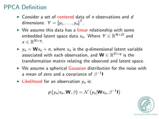
I Consider a set of centered data of n observations and d
dimensions: Y = [y1; : : : ; yn]T .
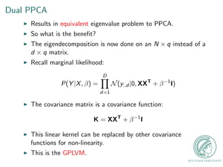
I We assume this data has a linear relationship with some
embedded latent space data xn. Where Y 2 RND and
x 2 RNq.
I yn = Wxn + n, where xn is the q-dimensional latent variable
associated with each observation, and W 2 RDq is the
transformation matrix relating the observed and latent space.
I We assume a spherical Gaussian distribution for the noise with
a mean of zero and a covariance of](https://image.slidesharecdn.com/gplvmpres-141023123617-conversion-gate01/85/The-Gaussian-Process-Latent-Variable-Model-GPLVM-18-320.jpg)

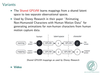

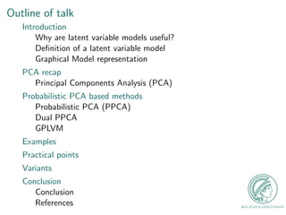
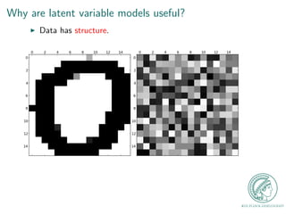
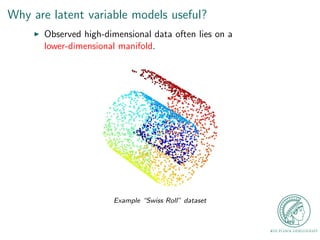
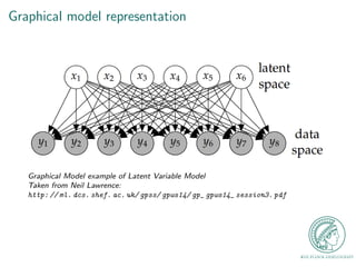
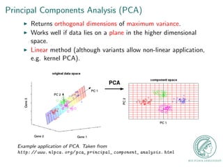
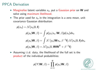
This document provides an outline for a talk on Gaussian Process Latent Variable Models (GPLVM). It begins with an introduction to why latent variable models are useful for dimensionality reduction. It then defines latent variable models and shows their graphical model representation. The document reviews PCA and introduces probabilistic versions like Probabilistic PCA (PPCA) and Dual PPCA. It describes how GPLVM generalizes these approaches using Gaussian processes. Examples applying GPLVM to face and motion data are provided, along with practical tips and an overview of GPLVM variants.


![[Kim+ ICML2012] Dirichlet Process with Mixed Random Measures : A Nonparametri...](https://cdn.slidesharecdn.com/ss_thumbnails/dp-mrmkimicml2012-120727233419-phpapp01-thumbnail.jpg?width=640&height=640&fit=bounds)