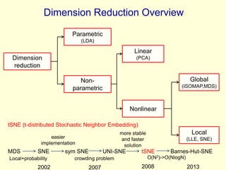
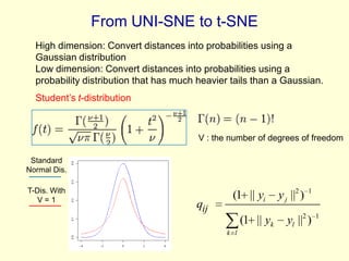
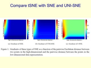
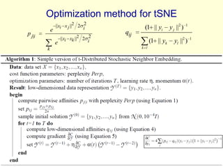
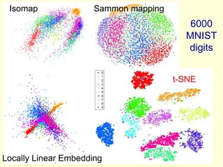
This document discusses t-Distributed Stochastic Neighbor Embedding (t-SNE), a technique for visualizing high-dimensional data. It begins by overviewing dimension reduction techniques before focusing on t-SNE. t-SNE is an improvement on Stochastic Neighbor Embedding (SNE) that converts similarities between data points to joint probabilities and minimizes the divergence between a high-dimensional and low-dimensional distribution. The document explains how t-SNE addresses issues like the "crowding problem" to better separate clusters in low dimensions. Optimization methods for t-SNE are also covered.

1. Visualization using tSNE
Yan Xu
Jun 7, 2013

2. Dimension Reduction Overview
Parametric
(LDA)
Linear
Dimension
reduction
(PCA)
Global
Nonparametric
(ISOMAP,MDS)
Nonlinear
tSNE (t-distributed Stochastic Neighbor Embedding)
easier
implementation
MDS
SNE
Local+probability
2002
Local
more stable
and faster
solution
sym SNE
UNI-SNE
crowding problem
2007
(LLE, SNE)
tSNE
Barnes-Hut-SNE
O(N2)->O(NlogN)
2008
2013

3. MDS: Multi-Dimensional Scaling
• Multi-Dimensional Scaling arranges the low-dimensional points so as to
minimize the discrepancy between the pairwise distances in the original
space and the pairwise distances in the low-D space.
Cost
(d ij
i j
d ij
|| xi
x j ||2
ˆ
d ij
|| yi
y j ||2
ˆ
d ij ) 2

4. Sammon mapping from MDS
high-D
distance
low-D
distance
|| xi x j || || y i y j ||
Cost
ij
2
|| xi x j ||
It puts too much emphasis on getting very small distances exactly
right. It’s slow to optimize and also gets stuck in different local
optima each time
Global to Local?

5. Maps that preserve local geometry
LLE (Locally Linear Embedding)
The idea is to make the local configurations of points in the low-dimensional
space resemble the local configurations in the high-dimensional space.
Cost
|| xi
i
wij x j || 2 ,
j N (i )
wij
1
j N (i )
fixed weights
Cost
|| y i
i
wij y j || 2
j N (i )
Find the y that minimize the cost subject to the constraint that the y have
unit variance on each dimension.

6. A probabilistic version of local MDS:
Stochastic Neighbor Embedding (SNE)
• It is more important to get local distances right than non-local ones.
• Stochastic neighbor embedding has a probabilistic way of deciding if
a pairwise distance is “local”.
• Convert each high-dimensional similarity into the probability that one
data point will pick the other data point as its neighbor.
probability of
p
picking j given i in j|i
high D
|| xi x j ||2 2 i2
e
|| xi xk ||2 2 i2
e
k
e
q j|i
|| yi y j ||2
e
k
2
|| yi yk ||
probability of
picking j given
i in low D

7. Picking the radius of the Gaussian that is
used to compute the p’s
• We need to use different radii in different parts of the space so that
we keep the effective number of neighbors about constant.
• A big radius leads to a high entropy for the distribution over
neighbors of i. A small radius leads to a low entropy.
• So decide what entropy you want and then find the radius that
produces that entropy.
• Its easier to specify perplexity:
||xi x j ||2 2 i2
e
p j|i
|| xi xk ||2 2 i2
e
k

8. The cost function for a low-dimensional
representation
Cost
KL ( Pi || Qi )
i
i
j
p j|i log
p j|i
q j|i
Gradient descent:
C
yi
2
(y j
y i ) ( p j|i
q j|i
j
Gradient update with a momentum term:
Learning
rate
Momentum
pi| j
qi| j )

9. Simpler version SNE: Turning conditional
probabilities into pairwise probabilities
pij
e
|| xi x j ||2 2 2
e
p j|i
pij
|| xk xl ||2 2 2
2n
k l
pij
j
Cost
KL( P || Q )
C
yi
4
( pij
j
pij log
qij )( yi
pi| j
yj)
pij
qij
1
2n

10. MNIST
Database
of handwritten
digits
28×28 images
Problem?

11. Why SNE does not have gaps between
classes
Crowding problem: the area accommodating moderately distant
datapoints is not large enough compared with the area
accommodating nearby datapoints.
A uniform background model (UNI-SNE) eliminates this effect and
allows gaps between classes to appear.
qij can never fall below
2
n(n 1)

13. From UNI-SNE to t-SNE
High dimension: Convert distances into probabilities using a
Gaussian distribution
Low dimension: Convert distances into probabilities using a
probability distribution that has much heavier tails than a Gaussian.
Student’s t-distribution
V : the number of degrees of freedom
Standard
Normal Dis.
T-Dis. With
V=1
qij
(1 || yi
(1 || yk
k l
y j ||2 )
1
yl ||2 )
1

14. Compare tSNE with SNE and UNI-SNE
18
16
14
12
14
12
10
10
-2
-4

15. Optimization method for tSNE
||xi x j ||2 2 i2
e
p j|i
e
k
|| xi xk ||2 2 i2
qij
(1 || yi
(1 || yk
k l
y j ||2 )
1
yl ||2 )
1

16. Optimization method for tSNE
Tricks:
1. Keep momentum term small until the map points have become
moderately well organized.
2. Use adaptive learning rate described by Jacobs (1988), which
gradually increases the learning rate in directions where the
gradient is stable.
3. Early compression: force map points to stay close together at the
start of the optimization.
4. Early exaggeration: multiply all the pij’s by 4, in the initial stages
of the optimization.

17. Isomap
Sammon mapping
6000
MNIST
digits
t-SNE
Locally Linear Embedding

18. tSNE vs Diffusion maps
Diffusion distance:
|| xi x j ||2
(1)
pij
e
n
Diffusion maps:
(
pijt )
(
pikt
k 1
1)
(
pkjt
1)

19. Weakness
1. It’s unclear how t-SNE performs on general dimensionality
reduction task;
2. The relative local nature of t-SNE makes it sensitive to the curse
of the intrinsic dimensionality of the data;
3. It’s not guaranteed to converge to a global optimum of its cost
function.

20. References:
t-SNE homepage:
http://homepage.tudelft.nl/19j49/t-SNE.html
Advanced Machine Learning: Lecture11: Non-linear Dimensionality Reduction
http://www.cs.toronto.edu/~hinton/csc2535/lectures.html
Plugin Ad: tSNE in Farsight
splot = new SNEPlotWindow(this);
splot->setPerplexity(perplexity);
splot->setModels(table, selection))
splot->show();