Download to read offline
![word2vec, node2vec, graph2vec, X2vec:
Towards a Theory of Vector Embeddings of
Structured Data
Martin Grohe
RWTH Aachen University
Vector representations of graphs and relational structures, whether hand-
crafted feature vectors or learned representations, enable us to apply standard
data analysis and machine learning techniques to the structures. A wide
range of methods for generating such embeddings have been studied in the
machine learning and knowledge representation literature. However, vector
embeddings have received relatively little attention from a theoretical point
of view.
Starting with a survey of embedding techniques that have been used in
practice, in this paper we propose two theoretical approaches that we see as
central for understanding the foundations of vector embeddings. We draw
connections between the various approaches and suggest directions for future
research.
Figure 1: Embedding graphs into a vector space
1
arXiv:2003.12590v1
[cs.LG]
27
Mar
2020
Wow](https://image.slidesharecdn.com/2003-240525122503-00da361b/85/word2vec-node2vec-graph2vec-X2vec-Towards-a-Theory-of-Vector-Embeddings-of-Structured-Data-NOTES-1-320.jpg)
![moreover, may be application dependent. However, this is not necessarily a problem,
because we can learn vector representations in such a way that they yield good results
when we use them to solve machine learning tasks (so-called downstream tasks). This
way, we never have to make the semantic relationships explicit. As a simple example, we
may use a nearest-neighbour based classification algorithm on the vectors our embedding
gives us; if it performs well then the distance between vectors must be relevant for this
classification task. This way, we can even use vector embeddings, trained to perform well
on certain machine learning tasks, to define semantically meaningful distance measures
on our original objects, that is, to define the distance distf (X, Y ) between objects X, Y ∈
X to be kf(X) − f(Y )k. We call distf the distance measure induced by the embedding
f.
In this paper, the objects X ∈ X we want to embed either are graphs, possibly
labelled or weighted, or more generally relational structures, or they are nodes of a
(presumably large) graph or more generally elements or tuples appearing in a relational
structure. When we embed entire graphs or structures, we speak of graph embeddings
or relational structure embeddings; when we embed only nodes or elements we speak
of node embeddings. These two types of embeddings are related, but there are clear
differences. Most importantly, in node embeddings there are explicit relations such as
adjacency and derived relations such as distance between the objects of X (the nodes
of a graph), whereas in graph embeddings all relations between objects are implicit or
“semantic”, for example “having the same number of vertices” or”having the same girth”
(see Figure 1).
The key theoretical questions we will ask about vector embeddings of objects in X are
the following.
Expressivity: Which properties of objects X ∈ X are represented by the embedding?
What is the meaning of the induced distance measure? Are there geometric prop-
erties of the latent space that represent meaningful relations on X?
Complexity: What is the computational cost of computing the vector embedding? What
are efficient embedding algorithms? How can we efficiently retrieve semantic in-
formation of the embedded data, for example, answer queries?
A third question that relates to both expressivity and complexity is what dimension to
choose for the latent space. In general, we expect a trade-off between (high) expressivity
and (low) dimension, but it may well be that there is an inherent dimension of the
data set. It is an appealing idea (see, for example, [98]) to think of “natural” data sets
appearing in practice as lying on a low dimensional manifold in high dimensional space.
Then we can regard the dimension of this manifold as the inherent dimension of the data
set.
Reasonably well-understood from a theoretical point of view are node embeddings of
graphs that aim to preserve distances between nodes, that is, embeddings f : V (G) → Rd
of the vertex set V (G) of some graph G such that distG(x, y) ≈ kf(x) − f(y)k, where
distG is the shortest-path distance in G. There is a substantial theory of such metric
3
Cool, not
just similarity](https://image.slidesharecdn.com/2003-240525122503-00da361b/85/word2vec-node2vec-graph2vec-X2vec-Towards-a-Theory-of-Vector-Embeddings-of-Structured-Data-NOTES-3-320.jpg)
![embeddings (see [64]). In many applications of node embeddings, metric embeddings are
indeed what we need.
However, the metric is only one aspect of the information carried by a graph or rela-
tional structure, and arguably not the most important one from a database perspective.
Moreover, if we consider graph embeddings rather than node embeddings, there is no
metric to start with. In this paper, we are concerned with structural vector embeddings
of graphs, relational structures, and their nodes. Two theoretical ideas that have been
shown to help in understanding and even designing vector embeddings of structures are
the Weisfeiler-Leman algorithm and various concepts in its context, and homomorphism
vectors, which can be seen as a general framework for defining “structural” (as opposed
to “metric”) embeddings. We will see that these theoretical concepts have a rich theory
that connects them to the embedding techniques used in practice in various ways.
The rest of the paper is organised as follows. Section 2 is a very brief survey of some
of the embedding techniques that can be found in the machine learning and knowledge
representation literature. In Section 3, we introduce the Weisfeiler-Leman algorithm.
This algorithm, originally a graph isomorphism test, turns out to be an important link
between the embedding techniques described in Section 2 and the theory of homomor-
phism vectors, which will be discussed in detail in Section 4. Finally, Section 5 is devoted
to a discussion of similarity measures for graphs and structures.
2 Embedding Techniques
In this section, we give a brief and selective overview of embedding techniques. More
thorough recent surveys are [50] (on node embeddings), [104] (on graph neural networks),
[102] (on knowledge graph embeddings), and [62] (on graph kernels).
2.1 From Metric Embeddings to Node Embeddings
Node embeddings can be traced back to the theory of embeddings of finite metric spaces
and dimensionality reduction, which have been studied in geometry (e.g. [21, 55]) and
algorithmic graph theory (e.g. [54, 64]). In statistics and data science, well-known tradi-
tional methods of metric embeddings and dimensionality reduction are multidimensional
scaling [63], Isomap [98], and Laplacian eigenmap [11]. More recent related approaches
are [1, 25, 85, 97]. The idea is always to embed the nodes of a graph in such a way that
the distance (or similarity) between vectors approximates the distance (or similarity) be-
tween nodes. Sometimes, this can be viewed as a matrix factorisation. Suppose we have
defined a similarity measure on the nodes of our graph G = (V, E) that is represented
by a similarity matrix S ∈ RV ×V . In the simplest version, we can just take S to be the
adjacency matrix of the graph; in the literature this is sometimes referred to a first-order
proximity. Another common choice is S = (Svw) with Svw := exp(−c distG(v, w)), where
c > 0 is a parameter. We describe our embedding of V into Rd by a matrix X ∈ RV ×d
whose rows xv ∈ Rd are the images of the nodes. If we measure the similarity between
vectors x, y by their normalised inner product hx,yi
kxkkyk (this is known as the cosine sim-
ilarity), then our objective is to find a matrix X with normalised rows that minimises
4
OM course
SimRank](https://image.slidesharecdn.com/2003-240525122503-00da361b/85/word2vec-node2vec-graph2vec-X2vec-Towards-a-Theory-of-Vector-Embeddings-of-Structured-Data-NOTES-4-320.jpg)
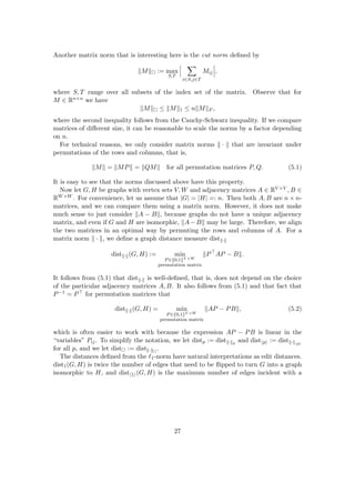
![(a)
(b)
(c)
Figure 2: Three node embeddings of a graph using (a) singular value decomposition of
adjacency matrix, (b) singular value decomposition of the similarity matrix
with entries Svw = exp(−2 dist(v, w)), (c) node2vec [48]
kXX> − SkF with respect to the Frobenius norm k · kF (or any other matrix norm, see
Section 5). In the basic version with the Frobenius norm, the problem can be solved
using the singular value decomposition of S. In a more general form, we compute a
similarity matrix b
S ∈ RV ×V whose (v, w)-entry quantifies the similarity between vec-
tors xv, xw and minimise the distance between S and b
S, for example using stochastic
gradient descent. In [50], this approach to learning node embeddings is described as an
encoder-decoder framework.
Learned word embeddings and in particular the word2vec algorithm [74] introduced
new ideas that had huge impact in natural language processing. These ideas also inspired
new approaches to node embeddings like DeepWalk [87] and node2vec [48] based on
taking short random walks in a graph and interpreting the sequence of nodes seen on such
random walks as if they were words appearing together in a sentence. These approaches
can still be described in the matrix-similarity (or encoder-decoder) framework: as the
similarity between nodes v and w we take the probability that a fixed-length random
walk starting in v ends in w. We can approximate this probability by sampling random
5
Unarguably, this looks the best](https://image.slidesharecdn.com/2003-240525122503-00da361b/85/word2vec-node2vec-graph2vec-X2vec-Towards-a-Theory-of-Vector-Embeddings-of-Structured-Data-NOTES-5-320.jpg)
![walks. Note that, even in undirected graphs, this similarity measure is not necessarily
symmetric.
From a deep learning perspective, the embedding methods described so far are all
“shallow” in that they directly optimise the output vectors and there are no hidden
layers; computing the vector xv corresponding to a node v amounts to a table lookup.
There are also deep learning methods for computing node embeddings (e.g. [26, 49, 101]).
Before we discuss such approaches any further, let us introduce graph neural networks
as a general deep learning framework for graphs that has received a lot of attention in
recent years.
2.2 Graph Neural Networks
When trying to apply deep learning methods to graphs or relational structures, we face
two immediate difficulties: (1) we want the methods to scale across different graph sizes,
but standard feed-forward neural networks have a fixed input size; (2) we want the
methods to be isomorphism invariant and not depend on a specific representation of the
input graph. Both points show that it is problematic to just feed the adjacency matrix
(or any other standard representation of a graph) into a deep neural network in a generic
“end-to-end” learning architecture.
Graph neural networks (GNNs) are a deep learning framework for graphs that avoids
both of these difficulties, albeit at the price of limited expressiveness (see Section 3).
Early forms of GNNs were introduced in [90, 36]; the version we present here is based on
[58, 49, 88]. Intuitively, a GNN model can be thought of as a message passing network
over the input graph G = (V, E). Each node v has a state xv ∈ Rd. Nodes can exchange
messages along the edges of G and update their states. To specify the model, we need
to specify two functions: an aggregation function that takes the current states of the
neighbours of a node and aggregates them into a single vector, and an update function
that takes the aggregate value obtained from the neighbours and the current state of the
node as inputs and computes the new state of the node. In a simple form, we may take
the following functions:
Aggregate : a(t+1)
v ←
X
w∈N(v)
Wagg · x(t)
w , (2.1)
Update : x(t+1)
v ← σ Wup ·
x
(t)
v
a
(t+1)
v
!!
, (2.2)
where Wagg ∈ Rc×d and Wup ∈ Rd×(c+d) are learned parameter matrices and σ is a
nonlinear “activation” function, for example the ReLU (rectified linear unit) function
σ(x) := max{0, x} applied pointwise to a vector. It is important to note that the
parameter matrices Wagg and Wup do not depend on the node v; they are shared across
all nodes of a graph. This parameter sharing allows it to use the same GNN model for
graphs of arbitrary sizes.
Of course, we can also use more complicated aggregation and update functions. We
only want these functions to be differentiable to be able to use gradient descent opti-
6](https://image.slidesharecdn.com/2003-240525122503-00da361b/85/word2vec-node2vec-graph2vec-X2vec-Towards-a-Theory-of-Vector-Embeddings-of-Structured-Data-NOTES-6-320.jpg)
![misation methods in the training phase, and we want the aggregation function to be
symmetric in its arguments x
(t)
w for w ∈ N(v) to make sure that the GNN computes a
function that is isomorphism invariant. For example, in [100] we use a linear aggregation
function and an update function computed by an LSTM (long short-term memory, [51]),
a specific recurrent neural network component that allows it to “remember” relevant in-
formation from the sequence x
(0)
v , x
(1)
v , . . . , x
(t)
v .
The computation of such a GNN model starts from a initial configuration x
(0)
v )v∈V
and proceeds through a fixed-number t of aggregation- and update-steps, resulting in a
final configuration x
(t)
v )v∈V . Note that this configuration gives us a node embedding
v 7→ x
(t)
v of the input graph. We can also stack several such GNN layers, each with its own
aggregation and activation function, on top of one another, using the final configuration
of each (but the last) layer as the initial configuration of the following layer and the
final configuration of the last layer as the node embedding. As initial states, we can take
constant vectors like the all-ones vector for each node, or we can assign a random initial
state to each node. We can also use the initial state to represent the node labels if the
input graph is labelled.
To train a GNN for computing a node-embedding, in principle we can use any of
the loss functions used by the embedding techniques described in Section 2.1. The
reader may wonder what advantage the complicated GNN architecture has over just
optimising the embedding matrix X (as the methods described in Section 2.1 do). The
main advantage is that the GNN method is inductive, whereas the previously described
methods are transductive. This means that a GNN represents a function that we can
apply to arbitrary graphs, not just to the graph it was originally trained on. So if the
graph changes over time and, for example, nodes are added, we do not have to re-train
the embedding, but just embed the new nodes using the GNN model we already have,
which is much more efficient. We can even apply the model to an entirely new graph
and still hope it gives us a reasonable embedding. The most prominent example of an
inductive node-embedding tool based on GNNs is GraphSage [49].
Let me close this section by remarking that GNNs are used for all kinds of machine
learning tasks on graphs and not only to compute node embeddings. For example, a GNN
based architecture for graph classification would plug the output of the GNN layer(s)
into a standard feedforward network (possibly consisting only of a single softmax layer).
2.3 Knowledge Graph and Relational Structure Embeddings
Node embeddings of knowledge graphs have also been studied quite intensely in recent
years, remarkably by a community that seems almost disjoint from that involved in the
node embedding techniques described in Section 2.1. What makes knowledge graphs
somewhat special is that they come with labelled edges (or, equivalently, many different
binary relations) as well as labelled nodes. It is not completely straightforward to adapt
the methods of Section 2.1 to edge- and vertex-labelled graphs. Another important
difference is in the objective function: the methods of Section 2.1 mainly focus on the
graph metric (even though approaches based on random walks like node2vec are flexible
7](https://image.slidesharecdn.com/2003-240525122503-00da361b/85/word2vec-node2vec-graph2vec-X2vec-Towards-a-Theory-of-Vector-Embeddings-of-Structured-Data-NOTES-7-320.jpg)
![and also incorporate structural criteria). However, shortest-path distance is less relevant
in knowledge graphs.
Rather than focussing on distances, knowledge graph embeddings focus on establishing
a correspondence between the relations of the knowledge graph and geometric relation-
ships in the latent space. A very influential algorithm, TransE [18] aims to associate
a specific translation of the latent space with each relation. Recall the example of the
introduction, where entities Paris, France, Santiago, Chile were supposed to be em-
bedded in such a way that xParis − xFrance ≈ xSantiago − xChile, so that the relation
is-capital-of corresponds to the translation by t := xParis − xFrance.
A different algorithm for mapping relations to geometric relationships is Rescal [83].
Here the idea is to associate a bilinear form βR with each relation R in such a way
that for all entities v, w it holds that βR(xv, xw) ≈ 1 if (v, w) ∈ R and βR(xv, xw) ≈ 0
if (v, w) 6∈ R. We can represent such a bilinear form βR by a matrix BR such that
βR(x, y) = x>BRy. Then the objective is to minimise, simultaneously for all R, the
term kXBRX> − ARk, where X is the embedding matrix with rows xv and AR is the
adjacency matrix of the relation R. Note that this is a multi-relational version of the
matrix-factorisation approach described in Section 2.1, with the additional twist that we
also need to find the matrix BR for each relation R.
Completing our remarks on knowledge graph embeddings, we mention that it is fairly
straightforward to generalise the GNN based node embeddings to (vertex- and edge-
)labelled graphs and hence to knowledge graphs [91].
While there is a large body of work on embedding knowledge graphs, that is, binary
relational structures, not much is known about embedding relations of higher arities. Of
course one approach to embedding relational structures of higher arities is to transform
them into their binary incidence structures (see Section 4.2 for a definition) and then
embed these using any of the methods available for binary structures. Currently, I
am not aware of any empirical studies on the practical viability of this approach. An
alternative approach [16, 17] is based on the idea of treating the rows of a table, that is,
tuples in a relation, like sentences in natural language and then use word embeddings
to embed the entities.
2.4 Graph Kernels
There are machine learning methods that operate on vector representations of their
input objects, but only use these vector representations implicitly and never actually
access the vectors. All they need to access is the inner product between two vectors.
For reasons that will become apparent soon, such methods are known as kernel methods.
Among them are support vector machines for classification [29] and principal component
analysis as well as k-means clustering for unsupervised learning [92] (see [93, Chapter 16]
for background).
A kernel functions for a set X of objects is a binary function K : X × X → R that
is symmetric, that is, K(x, y) = K(y, x) for all x, y ∈ X, and positive semidefinite, that
is, for all n ≥ 1 and all x1, . . . , xn ∈ X the matrix M with entries Mij := K(xi, xj) is
positive semidefinite. Recall that a symmetric matrix M ∈ Rn×n is positive semidefinite
8](https://image.slidesharecdn.com/2003-240525122503-00da361b/85/word2vec-node2vec-graph2vec-X2vec-Towards-a-Theory-of-Vector-Embeddings-of-Structured-Data-NOTES-8-320.jpg)
![if all its eigenvalues are nonnegative, or equivalently, if xT Mx ≥ 0 for all x ∈ Rn. It
can be shown that a symmetric function K : X × X → R is a kernel function if and only
if there is a vector embedding f : X → H of X into some Hilbert space H such that K
is the mapping induced by the inner product of H, that is, K(x, y) = hf(x), f(y)i for
all x, y ∈ X (see [93, Lemma 16.2] for a proof). For our purposes, it suffices to know
that a Hilbert space is a potentially infinite dimensional real vector space H with a a
symmetric bilinear form h·, ·i : H × H → R satisfying hx, xi > 0 for all x ∈ H {0}. A
difference between the embeddings underlying kernels and most other vector embeddings
is that the kernel embeddings usually embed into higher dimensional spaces (even infinite
dimensional Hilbert spaces). Dimension does not play a big role for kernels, because the
embeddings are only used implicitly. Nevertheless, it can sometimes be more efficient to
use the embeddings underlying kernels explicitly [61].
Kernel methods have dominated machine learning on graphs for a long time and,
despite of the recent successes of GNNs, they are still competitive. Quoting [62], “It
remains a current challenge in research to develop neural techniques for graphs that are
able to learn feature representations that are clearly superior to the fixed feature spaces
used by graph kernels.”
The first dedicated graph kernels were the random walk graph kernels [37, 56] based on
counting walks of all lengths. In some sense, they are similar to the random walk based
node-embedding algorithms described in Section 2.1. Other graph kernels are based on
counting shortest paths, trees and cycles, and small subgraph patterns [20, 52, 89, 95].
The important Weisfeiler-Leman kernels [94], which we will describe in Section 3, are
based on aggregating local neighbourhood information. All these kernels are defined for
graphs with discrete labels. The techniques, all essentially based on counting certain
subgraphs, are not directly applicable to graphs with continuous labels such as edge
weights. An adaptation to continuous labels based on hashing is proposed in [77].
Let me remark that there are also node kernels defined on the nodes of a graph
[60, 82, 96]. They implicitly give a vector embedding of the nodes. However, compared
to the node embedding techniques discussed before, they only play a minor role. For
graph embeddings, we are in the opposite situation: kernels are the dominant technique.
However, there are a few other approaches.
2.5 Graph Embeddings
Graph2Vec [80] is a transductive approach to embedding graphs inspired by word2vec
and some of the node embedding techniques discussed in Section 2.1. As before, “trans-
ductive” means that the embedding is computed for a fixed set of graphs in form of an
embedding matrix (or look-up table) and thus it only yields an embedding for graphs
known at training time. For typical machine learning applications it is unusual to op-
erate on set of graphs that is fixed in advance, so inductive embedding approaches are
clearly preferable.
GNNs can also be used to embed entire graphs, in the simplest form by just aggregating
the embeddings of the nodes computed by the GNN. Graph autoencoders [59, 86] give
a way to train such graph embeddings in an unsupervised manner. A more advanced
9](https://image.slidesharecdn.com/2003-240525122503-00da361b/85/word2vec-node2vec-graph2vec-X2vec-Towards-a-Theory-of-Vector-Embeddings-of-Structured-Data-NOTES-9-320.jpg)
![GNN architecture for learning graph embedding, based on capsule neural networks, is
proposed in [105].
3 The Weisfeiler-Leman Algorithm
We slightly digress from our main theme and introduce the Weisfeiler-Leman algorithm,
a very efficient combinatorial partitioning algorithm that was originally introduced as a
fingerprinting technique for chemical molecules [75]. The algorithm plays an important
role in the graph isomorphism literature, both in theory (for example, [7, 41]) and
practice, where it appears as a subroutine in all competitive graph isomorphism tools
(see [73]). As we will see, the algorithm has interesting connections with the embedding
techniques discussed in the previous section.
3.1 1-Dimensional Weisfeiler-Leman
The Weisfeiler-Leman algorithm has a parameter k, its dimension. We start by de-
scribing the 1-dimensional version 1-WL, which is also known as colour refinement or
naive vertex classification. The algorithm computes a partition of the nodes of its input
graph. It is convenient to think of the classes of the partition as colours of the nodes.
A colouring (or partition) is stable if any two nodes v, w of the same colour c have the
same number of neighbours of any colour d. The algorithm computes a stable colouring
by iteratively refining an initial colouring as described in Algorithm 1. Figure 3 shows
an example run of 1-WL. The algorithm is very efficient; it can be implemented to run
in time O((n + m) log n), where n is the number of vertices and m the number of edges
of the input graph [27]. Under reasonable assumptions on the algorithms used, this is
best possible [12].
1-WL
Input: Graph G
Initialisation: All nodes get the same colour.
Refinement Round: For all colours c in the current colouring and all nodes v, w of
colour c, the nodes v and w get different colours in the new colouring if there is
some colour d such that v and w have different numbers of neighbours of colour
d.
The refinement is repeated until the colouring is stable, then the stable colouring is
returned.
Algorithm 1: The 1-dimensional WL algorithm
To use 1-WL as an isomorphism test, we note that the colouring computed by the
algorithm is isomorphism invariant, which means that if we run the algorithm on two
isomorphic graphs the resulting coloured graphs will still be isomorphic and in particular
10](https://image.slidesharecdn.com/2003-240525122503-00da361b/85/word2vec-node2vec-graph2vec-X2vec-Towards-a-Theory-of-Vector-Embeddings-of-Structured-Data-NOTES-10-320.jpg)
![(a) initial graph (b) colouring after round 1
(c) colouring after round 2 (d) stable colouring after round 3
Figure 3: A run of 1-WL
have the same numbers of nodes of each colour. Thus, if we run the algorithm on two
graphs and find that they have distinct numbers of vertices of some colour, we have
produced a certificate of non-isomorphism. If this is the case, we say that 1-WL distin-
guishes the two graphs. Unfortunately, 1-WL does not distinguish all non-isomorphic
graphs. For example, it does not distinguish a cycle of length 6 from the disjoint union
of two triangles. But, remarkably, 1-WL does distinguish almost all graphs, in a precise
probabilistic sense [8].
3.2 Variants of 1-WL
The version of 1-WL we have formulated is designed for undirected graphs. For directed
graphs it is better to consider in-neighbours and out-neighbours of nodes separately.
1-WL can easily be adapted to labelled graphs. If vertex labels are present, they can be
incorporated in the initial colouring: two vertices get the same initial colour if and only
if they have the same label(s). We can incorporate edge labels in the refinement rounds:
two nodes v and w get different colours in the new colouring if there is some colour d
and some edge label λ such that v and w have a different number of λ-neighbours of
colour d.
However, if the edge labels are real numbers, which we interpret as edge weights, or
more generally elements of an arbitrary commutative monoid, then we can also use the
following weighted version of 1-WL due to [44]. Instead of refining by the number of
edges into some colour, we refine by the sum of the edge weights into that colour. Thus
the refinement round of Algorithm 1 is modified as follows: for all colours c in the current
colouring and all nodes v, w of colour c, v and w get different colours in the new colouring
if there is some colour d such that
X
x of colour d
α(v, x) 6=
X
x of colour d
α(w, x), (3.1)
where α(x, y) denotes the weight of the edge from x to y, and we set α(x, y) = 0
11
Can we use this property for almost isomorphic graphs?](https://image.slidesharecdn.com/2003-240525122503-00da361b/85/word2vec-node2vec-graph2vec-X2vec-Towards-a-Theory-of-Vector-Embeddings-of-Structured-Data-NOTES-11-320.jpg)
![0.3 2 1 0 0.7
1 0 1 1 1
0.7 2 0 1 0.3
0
v1
v2
v3
w1 w2 w3 w4 w5
v1
v2
v3
w1
w2
w3
w4
w5
0.3
2
0
.
7
0
.
7
2
0.3
Figure 4: Stable colouring of a matrix and the corresponding weighted bipartite graph
computed by matrix WL
if there is no edge from x to y. This idea also allows us to define 1-WL on matri-
ces: with a matrix A ∈ Rm×n we associate a weighted bipartite graph with vertex set
{v1, . . . , vm, w1, . . . , wn} and edge weights α vi, wj) := Aij and α(vi, vi0 ) = α(wj, wj0 ) =
0 and run weighted 1-WL on this weighted graph with initial colouring that distinguishes
the vi (rows) from the wj (columns). An example is shown in Figure 4. This matrix-
version of WL was applied in [44] to design a dimension reduction techniques that speeds
up the solving of linear programs with many symmetries (or regularities).
3.3 Higher-Dimensional WL
For this paper, the 1-dimensional version of the Weisfeiler-Leman algorithm is the most
relevant, but let us briefly describe the higher dimensional versions. In fact, it is the
2-dimensional version, also referred to as classical WL, that was introduced by Weis-
feiler and Leman [103] in 1968 and gave the algorithm its name. The k-dimensional
Weisfeiler-Leman algorithm (k-WL) is based on the same iterative-refinement idea as 1-
WL. However, instead of vertices, k-WL colours k-tuples of vertices of a graph. Initially,
each k-tuple is “coloured” by the isomorphism type of the subgraph it induces. Then in
the refinement rounds, the colour information is propagated between “adjacent” tuples
that only differ in one coordinate (details can be found in [24]). If implemented using
similar ideas as for 1-WL, k-WL runs in time O(nk+1 log n) [53].
Higher-dimensional WL is much more powerful than 1-WL, but Cai, Fürer, and Im-
merman [24] proved that for every k there are non-isomorphic graphs Gk, Hk that are
not distinguished by k-WL. These graphs, known as the CFI graphs, have size O(k) and
are 3-regular.
DeepWL, a WL-Version of unlimited dimension that can distinguish the CFI-graphs
in polynomial time, was recently introduced in [47].
3.4 Logical and Algebraic Characterisations
The beauty of the WL algorithm lies in the fact that its expressiveness has several natural
and completely unrelated characterisations. Of these, we will see two in this section.
Later, we will see two more characterisations in terms of GNNs and homomorphism
12](https://image.slidesharecdn.com/2003-240525122503-00da361b/85/word2vec-node2vec-graph2vec-X2vec-Towards-a-Theory-of-Vector-Embeddings-of-Structured-Data-NOTES-12-320.jpg)
![numbers.
The logic C is the extension of first-order logic by counting quantifiers of the form
∃≥px (“there exists at least p elements x”). Every C-formula is equivalent to a formula
of plain first-order logic. However, here we are interested in fragments of C obtained
by restricting the number of variables of formulas, and the translation from C to first-
order logic may increase the number of variables. For every k ≥ 1, by Ck
we denote the
fragment of C consisting of all formulas with at most k (free or bound) variables. The
finite variable logics Ck
play an important role in finite model theory (see, for example,
[40]). Cai, Fürer, and Immerman [24] have related these fragments to the WL algorithm.
Theorem 3.1 ([24]). Two graphs are Ck+1
-equivalent, that is, they satisfy the same
sentences of the logic Ck+1
, if and only if k-WL does not distinguish the graphs.
Let us now turn to an algebraic characterisation of WL. Our starting point is the
observation that two graphs G, H with vertex sets V, W and adjacency matrices A ∈
RV ×V , B ∈ RW×W are isomorphic if and only there is a permutation matrix X ∈ RV ×W
such that X>AX = B. Recall that a permutation matrix is a {0, 1}-matrix that has
exactly one 1-entry in each row and in each column. Since permutation matrices are
orthogonal (i.e., they satisfy X> = X−1), we can rewrite this as AX = XB, which has
the advantage of being linear. This corresponds to the following linear equations in the
variables Xvw, for v ∈ V and w ∈ W:
X
v0∈V
Avv0 Xv0w =
X
w0∈W
Xvw0 Bw0w for all v ∈ V, w ∈ W. (3.2)
We can add equations expressing that the row and column sums of the matrix X are 1,
which implies that X is a permutation matrix if the Xvw are nonnegative integers.
X
w0∈W
Xvw0 =
X
v0∈V
Xv0w = 1 for all v ∈ V, w ∈ W. (3.3)
Obviously, equations (3.2) and (3.3) have a nonnegative integer solution if and only if
the graphs G and H are isomorphic. This does not help much from an algorithmic point
of view, because it is NP-hard to decide if a system of linear equations and inequalities
has an integer solution. But what about nonnegative rational solutions? We know that
we can compute them in polynomial time. A nonnegative rational solution to (3.2) and
(3.3), which can also be seen as a doubly stochastic matrix satisfying AX = XB, is
called a fractional isomorphism between G and H. If such a fractional isomorphism
exists, we say that G and H are fractionally isomorphic. Tinhofer [99] proved the
following theorem.
Theorem 3.2 ([99]). Graphs G and H are fractionally isomorphic if and only if 1-WL
does not distinguish G and H.
A corresponding theorem also holds for the weighted and the matrix version of 1-
WL [44]. Moreover, Atserias and Maneva [5] proved a generalisation that relates k-WL
13](https://image.slidesharecdn.com/2003-240525122503-00da361b/85/word2vec-node2vec-graph2vec-X2vec-Towards-a-Theory-of-Vector-Embeddings-of-Structured-Data-NOTES-13-320.jpg)
![G
C0
C1
C2
Figure 5: Viewing colours of WL as trees
to the level-k Sherali-Adams relaxation of the system of equations and thus yields an
algebraic characterisation of k-WL indistinguishability (also see [45, 71] and [6, 84, 13, 39]
for related algebraic aspects of WL).
Note that to decide whether two graphs G, H with adjacency matrices G, H are frac-
tionally isomorphic, we can minimise the convex function kAX −XBkF , where X ranges
over the convex set of doubly stochastic matrices. To minimise this function, we can
use standard gradient descent techniques for convex minimisation. It was shown in [57]
that, surprisingly, the refinement rounds of 1-WL closely correspond to the iterations of
the Frank-Wolfe convex minimisation algorithm.
3.5 Weisfeiler-Leman Graph Kernels
The WL algorithm collects local structure information and propagates it along the edges
of a graph. We can define very effective graph kernels based on this local information.
For every i ≥ 0, let Ci be the set of colours that 1-WL assigns to the vertices of a graph
in the i-th round. Figure 5 illustrates that we can identify the colours in Ci with rooted
trees of height i. For every graph G and every colour c ∈ Ci, by wl(c, G) we denote the
number of vertices that receive colour c in the ith round of 1-WL.
Example 3.3. For the graph G shown in Figure 5 we have
wl
, G
= 2, wl
, G
= 0.
For every t ∈ N, the t-round WL-kernel is the mapping K
(t)
WL defined by
K
(t)
WL(G, H) :=
t
X
i=0
X
c∈Ci
wl(c, G) · wl(c, H)
for all graphs G, H. It is easy to see that this mapping is symmetric and positive-
semidefinite and thus indeed a kernel mapping; the corresponding vector embedding
maps each graph G to the vector
wl(c, G) c ∈
t
[
i=0
Ci
.
14](https://image.slidesharecdn.com/2003-240525122503-00da361b/85/word2vec-node2vec-graph2vec-X2vec-Towards-a-Theory-of-Vector-Embeddings-of-Structured-Data-NOTES-14-320.jpg)
![Note that formally, we are mapping G to an infinite dimensional vector space, because
all the sets Ci for i ≥ 1 are infinite. However, for a graph G of order n the vector as at
most kn + 1 nonzero entries. We can also define a version KWL of the WL-kernel that
does not depend on a fixed-number of rounds by letting
KWL(G, H) :=
X
i≥0
1
2i
X
c∈Ci
wl(c, G) · wl(c, H).
The WL-kernel was introduced by Shervashidze et al. [94] under the name Weisfeiler-
Leman subtree kernel. They also introduce variants such as a Weisfeiler-Leman shortest
path kernel. A great advantage the WL (subtree) kernel has over most of the graph
kernels discussed in Section 2.4 is its efficiency, while performing at least as good as
other kernels on downstream tasks. Shervashidze et al. [94] report that in practice, t = 5
is a good number of rounds for the t-round WL-kernel.
There are also graph kernels based on higher dimensional WL algorithm [76].
3.6 Weisfeiler-Leman and GNNs
Recall that a GNN computes a sequence (x
(t)
v )v∈V , for t ≥ 0, of vector embeddings of a
graph G = (V, E). In the most general form, it is recursively defined by
x(t+1)
v = fUP
x(t)
v , fAGG xw w ∈ N(v)
,
where the aggregation function fAGG is symmetric in its arguments. It has been observed
in several places [49, 78, 106] that this is very similar to the update process of 1-WL.
Indeed, it is easy to see that if the initial embedding x
(0)
v is constant then for any two
vertices v, w, if 1-WL assigns the same colour to v and w then x
(t)
v = x
(t)
w . This implies
that two graphs that cannot be distinguished by 1-WL will give the same result for any
GNN applied to them; that is, GNNs are at most as expressive as 1-WL. It is shown in
[78] that a converse of this holds as well, even if the aggregation and update functions
of the GNN are of a very simple form (like (2.1) and (2.2) in Section 2.2). Based on
the connection between WL and logic, a more refined analysis of the expressiveness of
GNNs was carried out in [10]. However, the limitations of the expressiveness only hold
if the initial embedding x
(0)
v is constant (or at least constant on all 1-WL colour classes).
We can increase the expressiveness of GNNs by assigning random initial vectors x
(0)
v
to the vertices. The price we pay for this increased expressiveness is that the output
of a run of the GNN model is no longer isomorphism invariant. However, the whole
randomised process is still isomorphism invariant. More formally, the random variable
that associates an output x
(0)
v )v∈V with each graph G is isomorphism invariant.
A fully invariant way to increase the expressiveness of GNNs is to build “higher-
dimensional” GNNs, inspired by the higher-dimensional WL algorithm. Instead of nodes
of the graphs, they operate on constant sized tuples or sets of vertices. A flexible
architecture for such higher-dimensional GNNs is proposed in [78].
15](https://image.slidesharecdn.com/2003-240525122503-00da361b/85/word2vec-node2vec-graph2vec-X2vec-Towards-a-Theory-of-Vector-Embeddings-of-Structured-Data-NOTES-15-320.jpg)
![4 Counting Homomorphisms
Most of the graph kernels and also some of the node embedding techniques are based
on counting occurrences of substructures like walks, cycles, or trees. There are differ-
ent ways of embedding substructures into a graph. For example, walks and paths are
the same structures, but we allow repeated vertices in a walk. Formally, “walks” are
homomorphic images of path graphs, whereas “paths” are embedded path graphs. It
turns that homomorphisms and homomorphic images give us a very robust and flexible
“basis” for counting all kinds of substructures [30].
A homomorphism from a graph F to a graph G is a mapping h from the nodes of
F to the nodes of G such that for all edges uu0 of F the image h(u)h(u0) is an edge of
G. On labelled graphs, homomorphisms have to preserve vertex and edge labels, and on
directed graphs they have to preserve the edge direction. Of course we can generalise
homomorphisms to arbitrary relational structures, and we remind the reader of the close
connection between homomorphisms and conjunctive queries. We denote the number of
homomorphisms from F to G by hom(F, G).
Example 4.1. For the graph G shown in Figure 5 we have
hom
, G
= 18, hom
, G
= 114.
To calculate these numbers, we observe that for the star Sk (tree of height 1 with k
leaves) we have hom(Sk, G) =
P
v∈V (G) degG(v)k.
For every class F of graphs, the homomorphism counts hom(F, G) give a graph em-
bedding HomF defined by
HomF(G) := hom(F, G) F ∈ F
for all graphs G. If F is infinite, the latent space RF of the embedding HomF is an infinite
dimensional vector space. By suitably scaling the infinite series involved, we can define
an inner product on a subspace HF of RF that includes the range of HomF. This also
gives us a graph kernel. One way of making this precise is as follows. For every k, we
let Fk be the set of all F ∈ F of order |F| := |V (F)| = k. Then we let
KF(G, H) :=
∞
X
k=1
1
|Fk|
X
F∈Fk
1
kk
hom(F, G) · hom(F, H). (4.1)
There are various other ways of doing this, for example, rather than looking at the
sum over all F ∈ Fk we may look at the maximum. In practice, one will simply cut
off of the infinite series and only consider a finite subset of F. A problem with using
homomorphism vectors as graph embeddings is that the homomorphism numbers quickly
get tremendously large. In practice, we take logarithms of theses numbers, possibly
scaled by the size of the graphs from F. So, a practically reasonable graph embedding
16](https://image.slidesharecdn.com/2003-240525122503-00da361b/85/word2vec-node2vec-graph2vec-X2vec-Towards-a-Theory-of-Vector-Embeddings-of-Structured-Data-NOTES-16-320.jpg)
![based on homomorphism vectors would take a finite class F of graphs and map each G
to the vector 1
|F|
log hom(F, G)
F ∈ F
.
Initial experiments show that this graph embedding performs very well on downstream
classification tasks even if we take F to be a small class (of size 20) of graphs consisting
of binary trees and cycles. This is a good indication that homomorphism vectors extract
relevant features from a graph. Note that the size of the class F is the dimension of the
feature space.
Apart from these practical considerations, homomorphisms vectors have a beautiful
theory that links them to various natural notions of similarity between structures, in-
cluding indistinguishability by the Weisfeiler-Leman algorithm.
4.1 Homomorphism Indistinguishability
Two graphs G and H are homomorphism-indistinguishable over a class F of a graphs if
HomF(G) = HomF(H). Lovász proved that homomorphism indistinguishability over the
class G of all graphs corresponds to isomorphism.
Theorem 4.2 ([65]). For all graphs G and H,
HomG(G) = HomG(H) ⇐⇒ G and H are isomorphic.
Proof. The backward direction is trivial. For the forward direction, suppose that HomG(G) =
HomG(H), that is, for all graphs F it holds that hom(F, G) = hom(F, H).
We can decompose every homomorphism h : F → F0 as h = f ◦ g such that for some
graph F00:
• g : F → F00 is an epimorphism, that is, a homomorphism such that for every
v ∈ V (F00) there is a u ∈ V (F) with g(u) = v and for every vv0 ∈ E(F00) there is
a uu0 ∈ E(F) with g(u) = v and g(u0) = v0;
• f : F00 → F0 is an embedding (or monomorphism), that is, a homomorphism such
that f(u) 6= f(u0) for all u 6= u0.
Note that the graph F00 is isomorphic to the image h(F) and thus unique up to isomor-
phism. Moreover, there are precisely
aut(F00
) = number of automorphisms of F00
isomorphisms from F00 to h(F). This means that there are aut(F00) pairs (f, g) such that
h = f ◦ g and g : F → F00 is an epimorphism and f : F00 → F0 is an embedding. Thus
we can write
hom(F, F0
) =
X
F00
1
aut(F00)
· epi(F, F00
) · emb(F00
, F0
), (4.2)
where epi(F, F00) is the number of epimorphisms from F onto F00, emb(F00, F0) is the
number of embeddings of F00 into F0, and the sum ranges over all isomorphism types of
17](https://image.slidesharecdn.com/2003-240525122503-00da361b/85/word2vec-node2vec-graph2vec-X2vec-Towards-a-Theory-of-Vector-Embeddings-of-Structured-Data-NOTES-17-320.jpg)
![G H
Figure 6: Co-spectral graphs
graphs F00. Furthermore, as epi(F, F00) = 0 if |F00| |F|, we can restrict the sum to F00
of order |F00| ≤ |F|.
Let F1, . . . , Fm be an enumeration of all graphs of order at most n := max{|G|, |H|}
such that each graph of order at most n is isomorphic to exactly one graph in this list and
that i ≤ j implies |Fi| |Fj| or |Fi| = |Fj| and kFik := |E(Fi)| ≤ kFjk. Let HOM be the
matrix with entries HOM ij := hom(Fi, Fj), P the matrix with entries Pij := epi(Fi, Fj),
M the matrix with entries Mij := emb(Fi, Fj), and D the diagonal matrix with entries
Dii := 1
aut(Fi). Then (4.2) yields the following matrix equation;
HOM = P · D · M. (4.3)
The crucial observation is that P is an lower triangular matrix, because epi(Fi, Fj) 0
implies |Fi| ≥ |Fj| and kFik ≥ kFjk. Moreover, P has positive diagonal entries, because
epi(Fi, Fi) ≥ 1. Similarly, M is an upper triangular matrix with positive diagonal entries.
Thus P and M are invertible. The diagonal matrix D is invertible as well, because
Dii = aut(Fi) ≥ 1. Thus the matrix HOM is invertible.
As |G|, |H| ≤ n there are graphs Fi, Fj such that G is isomorphic to Fi and H is
isomorphic to Fj. Since hom(Fk, G) = hom(Fk, H) for all k by the assumption of the
lemma, the ith and jth column of HOM are identical. As HOM is invertible, this implies
that i = j and thus that G and H are isomorphic.
The theorem can be seen as a the starting point for the theory of graph limits [19, 67,
68]. The graph embedding HomG maps graphs into an infinite dimensional real vector
space, which can be turned into a Hilbert space by defining a suitable inner product.
This transformation enables us to analyse graphs with methods of linear algebra and
functional analysis and, for example, to consider convergent sequences of graphs and
their limits, called graphons (see [67]).
However, not only the “full” homomorphism vector HomG(G) of a graph G, but also
its projections HomF(G) to natural classes F capture very interesting information about
G. A first result worth mentioning is the following. This result is well-known, though
usually phrased differently. Two graphs are co-spectral if their adjacency matrices have
the same eigenvalues with the same multiplicities. Figure 6 shows two graph that are
co-spectral, but not isomorphic.
Theorem 4.3 (Folklore). For all graphs G and H,
HomC(G) = HomC(H) ⇐⇒ G and H are co-spectral.
Here C denotes the class of all cycles.
18](https://image.slidesharecdn.com/2003-240525122503-00da361b/85/word2vec-node2vec-graph2vec-X2vec-Towards-a-Theory-of-Vector-Embeddings-of-Structured-Data-NOTES-18-320.jpg)
![Proof sketch. Observe that for the cycle Ck of length k we have hom(Ck, G) := trace(Ak),
where A is the adjacency matrix of G. It is well-known that the trace of a symmetric real
matrix is the sum of its eigenvalues and that the eigenvalues of Ak are the kth powers
of the eigenvalues of A. This immediately implies the backward direction. By a simple
linear-algebraic argument, it also implies the forward direction.
Dvorák [33] proved that homomorphism counts of trees, and more generally, graphs
of bounded tree width link homomorphism vectors to the Weisfeiler-Leman algorithm.
Theorem 4.4 ([33]). For all graphs G and H and all k ≥ 1,
HomTk
(G) = HomTk
(H) ⇐⇒ k-WL does not distinguish G and H.
Here Tk denotes the class of all graphs of tree width at most k.
To prove the theorem, it suffices to consider connected graphs in Tk, because for a
graph F with connected components F1, . . . , Fm we have hom(F, G) =
Qm
i=1 hom(Fi, G).
The connected graphs of tree width 1 are the trees. We sketch a proof of the theorem
for trees in Section 4.4.
In combination with Theorem 3.2, Theorem 4.4 implies the following.
Corollary 4.5. For all graphs G and H,
HomT(G) = HomT(H) ⇐⇒ G and H are fraction-
ally isomorphic, that
is, equations (3.2) and
(3.3) have a nonnega-
tive rational solution.
Here T denotes the class of all trees.
Remarkably, for paths we obtain a similar characterisation that involves the same
equations, but drops the nonnegativity constraint.
Theorem 4.6 ([32]). For all graphs G and H,
HomP(G) = HomP(H) ⇐⇒ equations (3.2) and
(3.3) have a
rational solution.
Here P denotes the class of all paths.
While the proof of Theorem 4.4 relies on techniques similar to the proof of Theo-
rem 4.2, the proof of Theorem 4.3 is based on spectral techniques similar to the proof of
Theorem 4.3.
Example 4.7. For the co-spectral graphs G, H shown in Figure 6 we have
hom
, G
= 20, hom
, H
= 16.
Thus HomP(G) 6= HomP(H).
19](https://image.slidesharecdn.com/2003-240525122503-00da361b/85/word2vec-node2vec-graph2vec-X2vec-Towards-a-Theory-of-Vector-Embeddings-of-Structured-Data-NOTES-19-320.jpg)
![G H
Figure 7: Two graphs that are homorphism-indistinguishable over the class of paths
Example 4.8. Figure 7 shows graphs G, H with
HomP(G) = HomP(H).
Obviously, 1-WL distinguishes the two graphs. Thus HomT(G) 6= HomT(H). It can also
be checked that the graphs are not co-spectral. Hence HomC(G) 6= HomC(H)
Combined with Theorem 3.1, Theorem 4.4 implies the following correspondence be-
tween homomorphism counts of graphs of bounded tree width and the finite variable
fragments of the counting logic C introduced in Section 3.4.
Corollary 4.9. For all graphs G and H and all k ≥ 1,
HomTk
(G) = HomTk
(H) ⇐⇒ G and H are Ck+1
-equivalent.
This is interesting, because it shows that the homomorphism vector HomTk
(G) gives
us all the information necessary to answer queries expressed in the logic Ck+1
. Unfortu-
nately, the result does not tell us how to answer Ck+1
-queries algorithmically if we have
access to the vector HomTk
(G). To make the question precise, suppose we have oracle
access that allows us to obtain, for every graph F ∈ Tk, the entry hom(F, G) of the
homomorphism vector. Is it possible to answer a Ck+1
-query in polynomial time (either
with respect to data complexity or combined complexity)?
Arguably, from a logical perspective it is even more natural to restrict the quantifier
rank (maximum number of nested quantifiers) in a formula rather than the number of
variables. Let Ck be the fragment of C consisting of all formulas of quantifier rank at most
k. We obtain the following characterisation of Ck-equivalence in terms of homomorphism
vectors over the class of graphs of tree depth at most k. Tree depth, introduced by Nešetřil
and Ossona de Mendez [81], is another structural graph parameter that has received a
lot of attention in recent years (e.g. [9, 23, 28, 35, 34]).
Theorem 4.10 ([42]). For all graphs G and H and all k ≥ 1,
HomTDk
(G) = HomTDk
(H) ⇐⇒ G and H are Ck-.equivalent.
Here TDk denotes the class of all graphs of tree depth at most k.
Another very remarkable result, due to Mančinska and Roberson [72], states that two
graphs are homomorphism-indistinguishable over the class of all planar graphs if and
only if they are quantum isomorphic. Quantum isomorphism, introduced in [4], is a
complicated notion that is based on similar systems of equations as (3.2) and (3.3) and
their generalisation characterising higher-dimensional Weisfeiler-Leman indistinguisha-
bility, but with non-commutative variables ranging over the elements of a C∗-algebra.
20](https://image.slidesharecdn.com/2003-240525122503-00da361b/85/word2vec-node2vec-graph2vec-X2vec-Towards-a-Theory-of-Vector-Embeddings-of-Structured-Data-NOTES-20-320.jpg)
![4.2 Beyond Undirected Graphs
So far, we have only considered homomorphism indistinguishability on undirected graphs.
A few results are known for directed graphs. In particular, Theorem 4.2 directly extends
to directed graphs. Actually, we have the following stronger result, also due to Lovász
[66] (also see [14]).
Theorem 4.11 ([66]). For all directed graphs G and H,
HomDA(G) = HomDA(G) ⇐⇒ G and H are isomorphic.
Here DA denote the class of all directed acyclic graphs.
It is straightforward to extend Theorem 4.2, Theorem 4.4 (for the natural generali-
sation of the WL algorithms to relational structures), and Theorem 4.10 to arbitrary
relational structures. This is very useful for binary relational structures such as knowl-
edge graphs. But for relations of higher arity one may consider another version based
on the incidence graph of a structure.
Let σ = {R1, . . . , Rm} be a relational vocabulary, where Ri is a ki-ary relation symbol.
Let k be the maximum of the ki. We let σI := {E1, . . . , Ek, P1, . . . , Pm}, where the
Ei are binary and the Pj are unary relation symbols. With every σ-structure A =
(V (A), R1(A), . . . , Rm(A)) we associates a σI-structure AI called the incidence structure
of A as follows:
• the universe of AI is
V (AI) := V (A) ∪
m
[
i=1
(Ri, v1, . . . , vki
(v1, . . . , vki
) ∈ Ri(A) ;
• for 1 ≤ j ≤ k, the relation Ej(AI) consists of all pairs
vj, (Ri, v1, . . . , vki
)
for (Ri, v1, . . . , vki
) ∈ V (AI) with ki ≥ j;
• for 1 ≤ i ≤ m, the relation Pi consist of all (Ri, v1, . . . , vki
) ∈ V (AI).
With this encoding of general structures as binary incidence structures we obtain the
following corollary.
Corollary 4.12. For all σ-structures A and B, the following are equivalent.
(1) HomT(σI )(AI) = HomT(σI )(BI), where T(σI) denotes the class of all σI-structures
whose underlying (Gaifman) graph is a tree;
(2) AI and BI are not distinguished by 1-WL;
(3) AI and BI are C2
-equivalent.
21](https://image.slidesharecdn.com/2003-240525122503-00da361b/85/word2vec-node2vec-graph2vec-X2vec-Towards-a-Theory-of-Vector-Embeddings-of-Structured-Data-NOTES-21-320.jpg)
![Böker [14] gave a generalisation of Theorem 4.4 to hypergraphs that is also based on
incidence graphs.
In a different direction, we can generalise the results to weighted graphs. Let us
consider undirected graphs with real-valued edge weights. We can also view them as
symmetric matrices over the reals. Recall that we denote the weight of an edge uv by
α(u, v) and that weighted 1-WL refines by sums of edge weights (instead of numbers of
edges). Let F be an unweighted graph and G a weighted graph. For every mapping
h : V (F) → V (G) we let
wt(h) :=
Y
uu0∈E(F)
α(h(u), h(u0
)).
As α(v, v0) = 0 if and only if vv0 6∈ E(G), we have wt(h) 6= 0 if and only if h is a
homomorphism from F to G; the weight of this homomorphism is the product of the
weights of the edges in its image. We let
hom(F, G) :=
X
h:V (F)→V (G)
wt(h).
In statistical physics, such sum-product functions are known as partition functions. For
a class F of graphs, we let
HomF(G) := hom(F, G) F ∈ F
.
Theorem 4.13 ([22]). For all weighted graphs G and H, the following are equivalent.
(1) HomT(G) = HomT(H) (recall that T denotes the class of all trees);
(2) G and H are not distinguished by weighted 1-WL;
(3) equations (3.2) and (3.3) have a nonnegative rational solution.
4.3 Complexity
In general, counting the number of homomorphisms from a graph F to a graph G is a #P-
hard problem. Dalmau and Jonsson [31] proved that, under the reasonable complexity
theoretic assumption #W[1] 6= FPT from parameterised complexity theory, for all classes
F of graphs, computing hom(F, G) given a graph F ∈ F and an arbitrary graph G, is
in polynomial time if and only if F has bounded tree width. This makes Theorem 4.4
even more interesting, because the entries of a homomorphism vector HomF(G) are
computable in polynomial time precisely for bounded tree width classes.
However, the computational problem we are facing is not to compute individual entries
of a homomorphism vectors, but to decide if two graphs have the same homomorphism
vector, that is, if they are homomorphism indistinguishable. The characterisation the-
orems of Section 4.1 imply that homomorphism indistinguishability is polynomial-time
decidable over the classes P of paths, C of cycles, T of trees, Tk of graphs of tree width at
most k, TDk of tree depth at most k. Moreover, homomorphism indistinguishability over
22](https://image.slidesharecdn.com/2003-240525122503-00da361b/85/word2vec-node2vec-graph2vec-X2vec-Towards-a-Theory-of-Vector-Embeddings-of-Structured-Data-NOTES-22-320.jpg)
![the class of G of all graphs is decidable in quasi-polynomial time by Babai’s [7] celebrated
result that graph isomorphism is decidable in quasi-polynomial time. It was proved in
[15] that homomorphism indistinguishability over the class of complete graphs is com-
plete for the complexity class C=P, which implies that it is co-NP hard, and that there
is a polynomial time decidable class F of graphs of bounded tree width such that homo-
morphism indistinguishability over F is undecidable. Quite surprisingly, the fact that
quantum isomorphism is undecidable [4] implies that homomorphism distinguishability
over the class of planar graphs is undecidable.
4.4 Homomorphism Node Embeddings
So far, we have defined graph and structure embeddings based on homomorphism vec-
tors. But we can also use homomorphism vectors to define node embeddings. A rooted
graph is a pair (G, v) where G is a graph and v ∈ V (G). For two rooted graphs (F, u)
and (G, v), by hom(F, G; u 7→ v) we denote the number of homomorphism h from F to
G with h(u) = v. For a class F∗ of rooted graphs and a rooted graph (G, v), we let
HomF∗ (G, v) := hom(F, G; u 7→ v) (F, u) ∈ F∗
.
If we keep the graph G fixed, this gives us an embedding of the nodes of G into an infinite
dimensional vector space. Note that in the terminology of Section 2.1, this embedding is
“inductive” and not “transductive”, because it is not tied to a fixed graph. (Nevertheless,
the term “inductive” is not fitting very well here, because the embedding is not learned.)
In the same way we defined graph kernels based on homomorphism vectors of graphs,
we can now define node kernels.
It is straightforward to generalise Theorem 4.2 to rooted graphs, showing that for all
rooted graphs (G, v) and (H, w) it holds that
HomG∗ (G, v) = HomG∗ (H, w) ⇐⇒ there is an isopmor-
phism f from G to H
with f(v) = w.
Here G∗ denote the class of all rooted graphs. Maybe the easiest way to prove this is by
a reduction to node-labelled graphs.
Another key result of Section 4.1 that can be adapted to the node setting is Theo-
rem 4.4. We only state the version for trees.
Theorem 4.14. For all graphs G, H and all v ∈ V (G), w ∈ V (H), the following are
equivalent.
(1) HomT∗ (G, v) = HomT∗ (H, w) for the class T∗ of all rooted trees;
(2) 1-WL assigns the same colour to v and w.
This result is implicit in the proof of Theorem 4.4 (see [33, 32]). In fact, it can be
viewed as the graph theoretic core of the proof. We sketch the proof here and also show
how to derive Theorem 4.4 (for trees) from it.
23](https://image.slidesharecdn.com/2003-240525122503-00da361b/85/word2vec-node2vec-graph2vec-X2vec-Towards-a-Theory-of-Vector-Embeddings-of-Structured-Data-NOTES-23-320.jpg)
![Proof sketch. Recall from Section 3.5 that we can view the colours assigned by 1-WL
as rooted trees (see Figure 5). For the kth round of WL, this is a tree of height k, and
for the stable colouring we can view it as an infinite tree. Suppose now that the colour
of a vertex v of G is T. The crucial observation is that for every rooted tree (S, r) the
number hom(S, G; r 7→ v) is precisely the number of mappings h : V (S) → V (T) that
map the root r of S to the root of T and, for each node s ∈ V (S), map the children of
s to the children of h(s) in T. Let us call such mappings rooted tree homomorphisms.
Implication (2) =⇒ (1) follows directly from this observation. Implication (1) =⇒ (2)
follows as well, because by an argument similar to that used in the proof of Theorem 4.2
it can be shown that for distinct rooted trees T, T0 there is a rooted tree that has distinct
numbers of rooted tree homomorphisms to T, T0.
Corollary 4.15. For all graphs G, H and all v ∈ V (G), w ∈ V (H), the following are
equivalent.
(1) HomT∗ (G, v) = HomT∗ (H, w);
(2) for all formulas ϕ(x) of the logic C2
,
G |= ϕ(v) ⇐⇒ H |= ϕ(w).
Note that the node embeddings based on homomorphism vectors are quite different
from the node embeddings described in Section 2.1. They are solely based on structural
properties and ignore the distance information. Results like Corollary 4.15 show that the
structural information captured by the homomorphism-based embeddings in principle
enables us to answer queries directly on the embedding, which may be more useful than
distance information in database applications.
We close this section by sketching how Theorem 4.4 (for trees) follows from Theo-
rem 4.14.
Proof sketch of Theorem 4.4 (for trees). Let G, H be graphs. We need to prove
HomT(G) = HomT(H) ⇐⇒ 1-WL does not distinguish G and H. (4.4)
Without loss of generality we assume that V (G) ∩ V (H) = ∅. For x, y ∈ V (G) ∪ V (H),
we write x ∼ y if 1-WL assigns the same colour to x and y. By Theorem 4.14, for
X, Y ∈ {G, H} and x ∈ V (X), y ∈ V (Y ) we have x ∼ y if and only if HomT∗ (X, x) =
HomT∗ (X, y). Let R1, . . . , Rn be the ∼-equivalence classes, and for every j, let Pj :=
Rj ∩ V (G) and Qj := Rj ∩ V (H). Furthermore, let pj := |Pj| and qj := |Qj|.
We first prove the backward direction of (4.4). Assume that 1-WL does not distinguish
G and H. Then pj = qj for all j ∈ [n]. Let T be a tree, and let t ∈ V (T). Let
24](https://image.slidesharecdn.com/2003-240525122503-00da361b/85/word2vec-node2vec-graph2vec-X2vec-Towards-a-Theory-of-Vector-Embeddings-of-Structured-Data-NOTES-24-320.jpg)
![hj := hom(T, X; t 7→ x) for x ∈ Rj and X ∈ {G, H} with x ∈ V (X). Then
hom(T, G) =
X
v∈V (G)
hom(T, G; t 7→ v)
=
n
X
j=1
pjhj =
n
X
j=1
qjhj
=
X
w∈V (H)
hom(T, H; t 7→ w) = hom(T, H).
Since T was arbitrary, this proves HomT(G) = HomT(H).
The proof of the forward direction of (4.4) is more complicated. Assume HomT(G) =
HomT(H). There is a finite collection of m ≤ n
2
rooted trees (T1, r1), . . . , (Tm, rm) such
that for all X, Y ∈ {G, H} and x ∈ V (X), y ∈ V (Y ) we have x ∼ y if and only if for all
i ∈ [m],
hom(Ti, X; ri 7→ x) = hom(Ti, Y ; ri 7→ y).
Let aij := hom(Ti, X; ri 7→ x) for x ∈ Rj and X ∈ {G, H} with x ∈ V (X). Then for all
i we have
n
X
j=1
aijpj = hom(Ti, G) = hom(Ti, H) =
n
X
j=1
aijqj
Unfortunately, the matrix A = (aij)i∈[m],j∈[n] is not necessarily invertible, so we cannot
directly conclude that pj = qj for all j. All we know is that for any two columns of the
matrix there is a row such that the two columns have distinct values in that row. It turns
out that this is sufficient. For every vector d = (d1, . . . , dm) of nonnegative integers, let
(T(d), r(d)) be the rooted tree obtained by taking the disjoint union of di copies of Ti for
all i and then identifying the roots of all these trees. It is easy to see that
hom(T(d)
, X; r(d)
7→ x) =
m
Y
i=1
hom(Ti, X; ri 7→ x).
Thus, letting a
(d)
j :=
Qm
i=1 adi
ij , we have
n
X
j=1
a
(d)
j pj = hom(T(d)
, G) = hom(T(d)
, H) =
n
X
j=1
a
(d)
j qj.
Using these additional equations, it can be shown that pj = qj for all j (see [43,
Lemma 4.2]). Thus WL does not distinguish G and H.
4.5 Homomorphisms and GNNs
We have a correspondence between homomorphism vectors and and the Weisfeiler-Leman
algorithm (Theorems 4.4 and 4.14) and between the the WL algorithm and GNNs (see
Section 3.6). This also establishes a correspondence between homomorphism vectors and
GNNs. More directly, the correspondence between GNNs and homomorphism counts is
also studied in [69].
25](https://image.slidesharecdn.com/2003-240525122503-00da361b/85/word2vec-node2vec-graph2vec-X2vec-Towards-a-Theory-of-Vector-Embeddings-of-Structured-Data-NOTES-25-320.jpg)
![single vertex we need to flip to turn G into a graph isomorphic to H. Formally,
dist1(G, H) = 2 min
f:V →W
bijection
f(v)f(v0
) vv0
∈ E(G) 4E(H) . (5.3)
disth1i(G, H) =
min
f:V →W
bijection
max
v∈V
f(v0
) v0
∈ NG(v) 4
w0
w ∈ NH(f(v)) . (5.4)
Here 4 denotes the symmetric difference. Equation (5.3) is obvious; the factor ’2’
comes from the fact that we regard (undirected) edges as 2-element sets and not as
ordered pairs. To prove (5.4), we observe that for every matrix M ∈ Rn×n it holds that
kMkh1i = maxj∈[n]
Pn
i=1 |Mij|.
Despite these intuitive interpretations, it is debatable how much “semantic relevance”
these distance measures have. How similar are two graphs that can be transformed into
each other by flipping, say, 5% of the edges? Again, the answer to this question may
depend on the application context.
A big disadvantage the graph distance measures based on matrix norms have is that
computationally they are highly intractable (see, for example, [3] and the references
therein). It is even NP-hard to compute the distance between two trees (see [46] for
Frobenius distance and [38] for the distances based on operator norms), and distances
are hard to approximate. The problem of computing these distances is related to the
maximisation version of the quadratic assignment problem (see [70, 79]), a notoriously
hard combinatorial optimisation problem. Better behaved is the cut-distance dist; at
least it can be approximated within a factor of 2 [2].
The main source of hardness is the minimisation over the unwieldy set of all permuta-
tions (or permutation matrices). To alleviate this hardness, we can relax the integrality
constraints and minimise over the convex set of all doubly stochastic matrices instead.
That is, we define a relaxed distance measure
g
distk·k(G, H) = min
X∈{0,1}V ×W
doubly stochastic
kAX − XBk. (5.5)
Note that g
distk·k is only a pseudo-metric: the distance between nonisomorphic graphs
may be 0. Indeed, it follows from Theorem 3.2 that g
distk·k(G, H) = 0 if and only if G
and H are fractionally isomorphic. The advantage of these “relaxed” distances is that
for many norms k · k, computing g
distk·k is a convex minimisation problem that can be
solved efficiently.
So far, we have only discussed distance measures for graphs of the same order. To
extend these distance measures to arbitrary graphs, we can replace vertices by sets of
identical vertices in both graphs to obtain two graphs whose order is the least common
multiple of the orders of the two initial graphs (see [67, Section 8.1] for details).
Note that these matrix based similarity measures are only defined for (possibly weighted)
graphs. In particular for the operator norms, it is not clear how to generalise them to
relational structures, and if such a generalisation would even be meaningful.
28](https://image.slidesharecdn.com/2003-240525122503-00da361b/85/word2vec-node2vec-graph2vec-X2vec-Towards-a-Theory-of-Vector-Embeddings-of-Structured-Data-NOTES-28-320.jpg)
![5.2 Comparing Homomorphism Distances and Matrix Distances
It would be very nice if we could establish a connection between graph distance mea-
sures based on homomorphism vectors and those based on matrix norms. At least one
important result in this direction exists: Lovász [67] proves an equivalence between the
cut-distance of graphs and a distance measure derived from a suitably scaled homomor-
phism vector HomG.
It is tempting to ask if a similar correspondence can be established between g
distk·k
and HomF. There are many related question that deserve further attention.
6 Concluding Remarks
In this paper, we gave an overview of embeddings techniques for graphs and relational
structures. Then we discussed two related theoretical approaches, the Weisfeiler-Leman
algorithm with its various ramifications and homomorphism vectors. We saw that they
have a rich and beautiful theory that leads to new, generic families of vector embeddings
and helps us to get a better understanding of some of the techniques used in practice,
for example graph neural networks.
Yet we have also seen that we are only at the beginning and many questions remain
open, in particular when it comes to similarity measures defined on graphs and relational
structures.
From a database perspective, it will be important to generalise the embedding tech-
niques to relations of higher arities, which is not as trivial as it may seem (and where
surprisingly little has been done so far). A central question is then how to query the
embedded data. Which queries can we answer at all when we only see the vectors in
latent space? How do imprecisions and variations due to randomness affect the outcome
of such query answers? Probably, we can only answer queries approximately, but what
exactly is the semantics of such approximations? These are just a few questions that
need to be answered, and I believe they offer very exciting research opportunities for
both theoreticians and practitioners.
Acknowledgements
This paper was written in strange times during COVID-19 lockdown. I appreciate it
that some of my colleagues nevertheless took the time to answer various questions I
had on the topics covered here and to give valuable feedback on an earlier version of
this paper. In particular, I would like to thank Pablo Barceló, Neta Friedman, Benny
Kimelfeld, Christopher Morris, Petra Mutzel, Martin Ritzert, and Yufei Tao.
References
[1] A. Ahmed, N. Shervashidze, S. Narayanamurthy, V. Josifovski, and A.J. Smola.
Distributed large-scale natural graph factorization. In Proceedings of the 22nd
International World Wide Web Conference, pages 37–48, 2013.
29](https://image.slidesharecdn.com/2003-240525122503-00da361b/85/word2vec-node2vec-graph2vec-X2vec-Towards-a-Theory-of-Vector-Embeddings-of-Structured-Data-NOTES-29-320.jpg)
![[2] N. Alon and A. Naor. Approximating the cut-norm via Grothendieck’s inequality.
SIAM Journal on Computing, 35:787–803, 2006.
[3] V. Arvind, J. Köbler, S. Kuhnert, and Y. Vasudev. Approximate graph isomor-
phism. In B. Rovan, V. Sassone, and P. Widmayer, editors, Proceedings of the 37th
International Symposium on Mathematical Foundations of Computer Science, vol-
ume 7464 of Lecture Notes in Computer Science, pages 100–111. Springer Verlag,
2012.
[4] A. Atserias, Laura Mančinska, D.E. Roberson, R. Šámal, S. Severini, and
A. Varvitsiotis. Quantum and non-signalling graph isomorphisms. Journal of
Combinatorial Theory, Series B, 136:289–328, 2019.
[5] A. Atserias and E. Maneva. Sherali–Adams relaxations and indistinguishability in
counting logics. SIAM Journal on Computing, 42(1):112–137, 2013.
[6] A. Atserias and J. Ochremiak. Definable ellipsoid method, sums-of-squares proofs,
and the isomorphism problem. In Proceedings of the 33rd Annual ACM/IEEE
Symposium on Logic in Computer Science, pages 66–75, 2018.
[7] L. Babai. Graph isomorphism in quasipolynomial time. In Proceedings of the 48th
Annual ACM Symposium on Theory of Computing (STOC ’16), pages 684–697,
2016.
[8] L. Babai, P. Erdös, and S. Selkow. Random graph isomorphism. SIAM Journal
on Computing, 9:628–635, 1980.
[9] M. Bannach and T. Tantau. Parallel multivariate meta-theorems. In J. Guo and
D. Hermelin, editors, Proceedings of the 11th International Symposium on Pa-
rameterized and Exact Computation, volume 63 of LIPIcs, pages 4:1–4:17. Schloss
Dagstuhl - Leibniz-Zentrum für Informatik, 2016.
[10] P. Barceló, E.V. Kostylev, M. Monet, J. Pérez, J. Reutter, and J.P. Silva. The logi-
cal expressiveness of graph neural networks. In Proceedings of the 8th International
Conference on Learning Representations, 2020.
[11] M. Belkin and P. Niyogi. Laplacian eigenmaps for dimensionality reduction and
data representation. Neural Computation, 15(6):1373–1396, 2003.
[12] C. Berkholz, P. Bonsma, and M. Grohe. Tight lower and upper bounds for the com-
plexity of canonical colour refinement. Theory of Computing Systems, 60(4):581–
614, 2017.
[13] C. Berkholz and M. Grohe. Limitations of algebraic approaches to graph isomor-
phism testing. In M.M. Halldórsson, K. Iwama, N. Kobayashi, and B. Speckmann,
editors, Proceedings of the 42nd International Colloquium on Automata, Languages
and Programming, Part I, volume 9134 of Lecture Notes in Computer Science,
pages 155–166. Springer Verlag, 2015.
30](https://image.slidesharecdn.com/2003-240525122503-00da361b/85/word2vec-node2vec-graph2vec-X2vec-Towards-a-Theory-of-Vector-Embeddings-of-Structured-Data-NOTES-30-320.jpg)
![[14] J. Böker. Color refinement, homomorphisms, and hypergraphs. In I. Sau and
D.M. Thilikos, editors, Proceedings of the 45th International Workshop on Graph-
Theoretic Concepts in Computer Science, volume 11789 of Lecture Notes in Com-
puter Science, pages 338–350. Springer, 2019.
[15] J. Böker, Y. Chen, M. Grohe, and G. Rattan. The complexity of homomorphism
indistinguishability. In P. Rossmanith, P. Heggernes, and J.-P. Katoen, editors,
Proceedings of the 44th International Symposium on Mathematical Foundations of
Computer Science, volume 138 of Leibniz International Proceedings in Informatics
(LIPIcs), pages 54:1–54:13. Schloss Dagstuhl–Leibniz-Zentrum fuer Informatik,
2019.
[16] R. Bordawekar and O. Shmueli. Using word embedding to enable semantic queries
in relational databases. In Proceedings of the Data Management for End to End
Learning Work Workshop, SIGMOD’17, 2017.
[17] R. Bordawekar and O. Shmueli. Exploiting latent information in relational
databases via word embedding and application to degrees of disclosure. In Pro-
ceedings of the 9th Biennial Conference on Innovative Data Systems Research,
2019.
[18] A. Bordes, N. Usunier, A. Garcia-Duran, J. Weston, and O. Yakhnenko. Trans-
lating embeddings for modeling multi-relational data. In Advances in neural in-
formation processing systems, pages 2787–2795, 2013.
[19] C. Borgs, J. Chayes, L. Lovász, V. Sós, B. Szegedy, and K. Vesztergombi. Graph
limits and parameter testing. In Proceedings of the 38th Annual ACM Symposium
on Theory of Computing, pages 261–270, 2006.
[20] K.M. Borgwardt and H.-P. Kriegel. Shortest-path kernels on graphs. In Proceedings
of the 5th IEEE International Conference on Data Mining, pages 74–81, 2005.
[21] J. Bourgain. On Lipschitz embeddings of finite metric spaces in Hilbert spaces.
Israel Journal of Mathematics, 52(1-2):46–52, 1985.
[22] A. Bulatov, M. Grohe, and G. Rattan. In preparation.
[23] J. Bulian and A. Dawar. Graph isomorphism parameterized by elimination dis-
tance to bounded degree. In M. Cygan and P. Heggernes, editors, Proceedings of
the 9th International Symposium on Parameterized and Exact Computation, vol-
ume 8894 of Lecture Notes in Computer Science, pages 135–146. Springer Verlag,
2014.
[24] J. Cai, M. Fürer, and N. Immerman. An optimal lower bound on the number of
variables for graph identification. Combinatorica, 12:389–410, 1992.
[25] S. Cao, W. Lu, and Q. Xu. GraRep: Learning graph representations with global
structural information. In Proceedings of the 24th ACM International on Confer-
ence on Information and Knowledge Management, pages 891–900, 2015.
31](https://image.slidesharecdn.com/2003-240525122503-00da361b/85/word2vec-node2vec-graph2vec-X2vec-Towards-a-Theory-of-Vector-Embeddings-of-Structured-Data-NOTES-31-320.jpg)
![[26] S. Cao, W. Lu, and Q. Xu. Deep neural networks for learning graph representa-
tions. In Proceedings of the 30th AAAI Conference on Artificial Intelligence, pages
1145–1152, 2016.
[27] A. Cardon and M. Crochemore. Partitioning a graph in O(|A| log2 |V |). Theoretical
Computer Science, 19(1):85 – 98, 1982.
[28] Y. Chen and J. Flum. Tree-depth, quantifier elimination, and quantifier rank.
In Proceedings of the 33rd Annual ACM/IEEE Symposium on Logic in Computer
Science, pages 225–234, 2018.
[29] C. Cortes and V. Vapnik. Support-vector networks. Machine Learning, 20(3):273–
297, 1995.
[30] R. Curticapean, H. Dell, and D. Marx. Homomorphisms are a good basis for count-
ing small subgraphs. In Proceedings of the 49th Annual ACM SIGACT Symposium
on Theory of Computing (STOC ’17), pages 210–223, 2017.
[31] V. Dalmau and P. Jonsson. The complexity of counting homomorphisms seen from
the other side. Theoretical Computer Science, 329(1-3):315–323, 2004.
[32] H. Dell, M. Grohe, and G. Rattan. Lovász meets Weisfeiler and Leman. In
I. Chatzigiannakis, C. Kaklamanis, D. Marx, and D. Sannella, editors, Proceedings
of the 45th International Colloquium on Automata, Languages and Programming
(Track A), volume 107 of LIPIcs, pages 40:1–40:14. Schloss Dagstuhl - Leibniz-
Zentrum für Informatik, 2018.
[33] Z. Dvorák. On recognizing graphs by numbers of homomorphisms. Journal of
Graph Theory, 64(4):330–342, 2010.
[34] M. Elberfeld, M. Grohe, and T. Tantau. Where first-order and monadic second-
order logic coincide. ACM Transaction on Computational Logic, 17(4), 2016. Ar-
ticle No. 25.
[35] M. Elberfeld, A. Jakoby, and T. Tantau. Algorithmic meta theorems for circuit
classes of constant and logarithmic depth. In C. Dürr and T. Wilke, editors, Pro-
ceedings of the 29th International Symposium on Theoretical Aspects of Computer
Science, volume 14 of LIPIcs, pages 66–77. Schloss Dagstuhl - Leibniz-Zentrum
fuer Informatik, 2012.
[36] C. Gallicchio and A. Micheli. Graph echo state networks. In Proceedings of the
IEEE International Joint Conference on Neural Networks, 2010.
[37] T. Gärtner, P. Flach, and S. Wrobel. On graph kernels: Hardness results and
efficient alternatives. In Learning theory and kernel machines, pages 129–143.
Springer Verlag, 2003.
[38] T. Gervens. Spectral graph similarity. Master Thesis at RWTH Aachen, 2018.
32](https://image.slidesharecdn.com/2003-240525122503-00da361b/85/word2vec-node2vec-graph2vec-X2vec-Towards-a-Theory-of-Vector-Embeddings-of-Structured-Data-NOTES-32-320.jpg)
![[39] E. Grädel, M. Grohe, B. Pago, and W. Pakusa. A finite-model-theoretic view on
propositional proof complexity. Logical Methods in Computer Science, 15(1):4:1–
4:53, 2019.
[40] E. Grädel, P.G. Kolaitis, L. Libkin, M. Marx, J. Spencer, M.Y. Vardi, Y. Venema,
and S. Weinstein. Finite Model Theory and Its Applications. Springer Verlag,
2007.
[41] M. Grohe. Descriptive Complexity, Canonisation, and Definable Graph Structure
Theory, volume 47 of Lecture Notes in Logic. Cambridge University Press, 2017.
[42] M. Grohe. Counting bounded tree depth homomorphisms. ArXiv,
arXiv:2003.08164 [cs.LO], 2020.
[43] M. Grohe. Counting bounded tree depth homomorphisms. In Submitted, 2020.
[44] M. Grohe, K. Kersting, M. Mladenov, and E. Selman. Dimension reduction via
colour refinement. In A. Schulz and D. Wagner, editors, Proceedings of the 22nd
Annual European Symposium on Algorithms, volume 8737 of Lecture Notes in
Computer Science, pages 505–516. Springer-Verlag, 2014.
[45] M. Grohe and M. Otto. Pebble games and linear equations. Journal of Symbolic
Logic, 80(3):797–844, 2015.
[46] M. Grohe, G. Rattan, and G. Woeginger. Graph similarity and approximate iso-
morphism. In I. Potapov, P.G. Spirakis, and J. Worrell, editors, Proceedings of the
43rd International Symposium on Mathematical Foundations of Computer Science,
volume 117 of LIPIcs, pages 20:1–20:16. Schloss Dagstuhl - Leibniz-Zentrum für
Informatik, 2018.
[47] M. Grohe, P. Schweitzer, and D. Wiebking. Deep weisfeiler leman. ArXiv,
arXiv:2003.10935 [cs.LO], 2020.
[48] A. Grover and J. Leskovec. node2vec: Scalable feature learning for networks. In
B. Krishnapuram, M. Shah, A.J. Smola, C.C. Aggarwal, D. Shen, and R. Ras-
togi:, editors, Proceedings of the 22nd ACM SIGKDD International Conference on
Knowledge Discovery and Data Mining, pages 855–864, 2016.
[49] W. Hamilton, R. Ying, and J. Leskovec. Inductive representation learning on
large graphs. In Proceedings of the 30th Annual Conference on Neural Information
Processing Systems, pages 1024–1034, 2017.
[50] W.L. Hamilton, R. Ying, and J. Leskovec. Representation learning on graphs:
methods and applications. ArXiv, arXiv:1709.05584 [cs.SI], 2017.
[51] S. Hochreiter and J. Schmidhuber. Long short-term memory. Neural Computation,
9(8):1735–1780, 1997.
33](https://image.slidesharecdn.com/2003-240525122503-00da361b/85/word2vec-node2vec-graph2vec-X2vec-Towards-a-Theory-of-Vector-Embeddings-of-Structured-Data-NOTES-33-320.jpg)
![[52] T. Horváth, T. Gärtner, and S. Wrobel. Cyclic pattern kernels for predictive graph
mining. In Proceedings of the 10th ACM SIGKDD International Conference on
Knowledge Discovery and Data Mining, pages 158–167, 2004.
[53] N. Immerman and E. Lander. Describing graphs: A first-order approach to graph
canonization. In A. Selman, editor, Complexity theory retrospective, pages 59–81.
Springer-Verlag, 1990.
[54] P. Indyk. Algorithmic applications of low-distortion geometric embeddings. In
Proceedings of the 42nd IEEE Symposium on Foundations of Computer Science,
pages 10–33, 2001.
[55] W. Johnson and J. Lindenstrauss. Extensions of Lipschitz mappings into a Hilbert
space. Contemporary Mathematics, 26:189–206, 1984.
[56] H. Kashima, K. Tsuda, and A. Inokuchi. Marginalized kernels between labeled
graphs. In Proceedings of the 20th International Conference on Machine Learning,
pages 321–328, 2003.
[57] K. Kersting, M. Mladenov, R. Garnet, and M. Grohe. Power iterated color refine-
ment. In P. Stone C.E. Brodley, editor, Proceedings of the 28th AAAI Conference
on Artificial Intelligence, pages 1904–1910, 2014.
[58] T. N. Kipf and M. Welling. Semi-supervised classification with graph convolu-
tional networks. In Proceedings of the 5th International Conference on Learning
Representations, 2017.
[59] T.N. Kipf and M. Welling. Variational graph auto-encoders. ArXiv,
arXiv:1611.07308 [stat.ML], 2016.
[60] R. Kondor and J.D. Lafferty. Diffusion kernels on graphs and other discrete input
spaces. In Proceedings of the 19th International Conference on Machine Learning,
pages 315–322, 2002.
[61] N. Kriege, M. Neumann, C. Morris, K. Kersting, and P. Mutzel. A unifying view
of explicit and implicit feature maps of graph kernels. Data Mining and Knowledge
Discovery, 33(6):1505–1547, 2019.
[62] N.M. Kriege, F.D Johansson, and C. Morris. A survey on graph kernels. ArXiv,
arXiv:1903.11835 [cs.LG], 2019.
[63] J.B. Kruskal. Multidimensional scaling by optimizing goodness of fit to a nonmetric
hypothesis. Psychometrika, 29(1):1–27, 1964.
[64] N. Linial, E. London, and Y. Rabinovich. The geometry of graphs and some of its
algorithmic applications. Combinatorica, 15:212–245, 1995.
[65] L. Lovász. Operations with structures. Acta Mathematica Hungarica, 18:321–328,
1967.
34](https://image.slidesharecdn.com/2003-240525122503-00da361b/85/word2vec-node2vec-graph2vec-X2vec-Towards-a-Theory-of-Vector-Embeddings-of-Structured-Data-NOTES-34-320.jpg)
![[66] L. Lovász. On the cancellation law among finite relational structures. Periodica
Mathematica Hungarica, 1(2):145–156, 1971.
[67] L. Lovász. Large Networks and Graph Limits. American Mathematical Society,
2012.
[68] L. Lovász and B. Szegedy. Limits of dense graph sequences. Journal of Combina-
torial Theory, Series B, 96(6):933–957, 2006.
[69] T. Maehara and H. NT. A simple proof of the universality of invariant/equivariant
graph neural networks. ArXiv, arXiv:1910.03802 [cs.LG], 2019.
[70] K. Makarychev, R. Manokaran, and M. Sviridenko. Maximum quadratic assign-
ment problem: Reduction from maximum label cover and lp-based approximation
algorithm. ACM Transactions on Algorithms, 10(4):18, 2014.
[71] P. Malkin. Sherali–adams relaxations of graph isomorphism polytopes. Discrete
Optimization, 12:73–97, 2014.
[72] L. Mančinska and D.E. Roberson. Quantum isomorphism is equivalent to equality
of homomorphism counts from planar graphs. ArXiv, arXiv:1910.06958v2 [quant-
ph], 2019.
[73] B.D. McKay and A. Piperno. Practical graph isomorphism, II. Journal of Symbolic
Compututation, 60:94–112, 2014.
[74] T. Mikolov, I. Sutskever, K. Chen, G.S. Corrado, and J. Dean. Distributed repre-
sentations of words and phrases and their compositionality. In Proceedings of the
27th Annual Conference on Neural Information Processing Systems, pages 3111–
3119, 2013.
[75] H.L. Morgan. The generation of a unique machine description for chemical
structures—a technique developed at chemical abstracts service. Journal of Chem-
ical Documentation, 5(2):107–113, 1965.
[76] C. Morris, K. Kersting, and P. Mutzel. Globalized Weisfeiler-Lehman graph ker-
nels: Global-local feature maps of graphs. In Proceedings of the 2017 IEEE Inter-
national Conference on Data Mining, pages 327–336, 2017.
[77] C. Morris, N.M. Kriege, K. Kersting, and P. Mutzel. Faster kernel for graphs with
continuous attributes via hashing. In Proceedings of the 16th IEEE International
Conference on Data Mining, pages 1095–1100, 2016.
[78] C. Morris, M. Ritzert, M. Fey, W. Hamilton, J.E. Lenssen, G. Rattan, and
M. Grohe. Weisfeiler and leman go neural: Higher-order graph neural networks.
In Proceedings of the 33rd AAAI Conference on Artificial Intelligence, volume
4602-4609. AAAI Press, 2019.
35](https://image.slidesharecdn.com/2003-240525122503-00da361b/85/word2vec-node2vec-graph2vec-X2vec-Towards-a-Theory-of-Vector-Embeddings-of-Structured-Data-NOTES-35-320.jpg)
![[79] V. Nagarajan and M. Sviridenko. On the maximum quadratic assignment prob-
lem. In Proceedings of the twentieth Annual ACM-SIAM Symposium on Discrete
Algorithms, pages 516–524, 2009.
[80] A. Narayanan, M. Chandramohan, R. Venkatesan, L. Chen, Y. Liu, and S. Jaiswal.
graph2vec: Learning distributed representations of graphs. ArXiv (CoRR),
arXiv:1707.05005 [cs.AI], 2017.
[81] J. Nešetřil and P. Ossona de Mendez. Linear time low tree-width partitions and
algorithmic consequences. In Proceedings of the 38th ACM Symposium on Theory
of Computing, pages 391–400, 2006.
[82] M. Neumann, R. Garnett, and K. Kersting. Coinciding walk kernels: Parallel
absorbing random walks for learning with graphs and few labels. In Proceedings
of the 5th Asian Conference on Machine Learning, pages 357–372, 2013.
[83] M. Nickel, V. Tresp, and H.-P. Kriegel. A three-way model for collective learning
on multi-relational data. In Proceedings of the 28th International Conference on
Machine Learning, pages 809–816, 2011.
[84] R. O’Donnell, J. Wright, C. Wu, and Y. Zhou. Hardness of robust graph isomor-
phism, Lasserre gaps, and asymmetry of random graphs. In Proceedings of the 25th
Annual ACM-SIAM Symposium on Discrete Algorithms, pages 1659–1677, 2014.
[85] M. Ou, P. Cui, J. Pei, Z. Zhang, and W. Zhu. Asymmetric transitivity preserv-
ing graph embedding. In Proceedings of the 22nd ACM SIGKDD International
Conference on Knowledge Discovery and Data Mining, pages 1105–1114, 2016.
[86] S. Pan, R. Hu, G. Long, J. Jiang, L. Yao, and C. Zhang. Adversarially regular-
ized graph autoencoder for graph embedding. ArXiv (CoRR), arXiv:1802.04407
[cs.LG], 2018.
[87] B. Perozzi, R. Al-Rfou, and S. Skiena. Deepwalk: Online learning of social rep-
resentations. In Proceedings of the 20th ACM SIGKDD International Conference
on Knowledge Discovery and Data Mining, pages 710–710, 2014.
[88] T. Pham, T. Tran, D. Phung, and S. Venkatesh. Column networks for collective
classification. In Proceedings of the 31st AAAI Conference on Artificial Intelli-
gence, pages 2485–2491, 2017.
[89] J. Ramon and T. Gärtner. Expressivity versus efficiency of graph kernels. In
Proceedings of the 1st International Workshop on Mining Graphs, Trees and Se-
quences, pages 65–74, 2003.
[90] F. Scarselli, M. Gori, A.C. Tsoi, M. Hagenbuchner, and G. Monfardini. The graph
neural network model. IEEE Transactions on Neural Networks, 20(1):61–80, 2009.
36](https://image.slidesharecdn.com/2003-240525122503-00da361b/85/word2vec-node2vec-graph2vec-X2vec-Towards-a-Theory-of-Vector-Embeddings-of-Structured-Data-NOTES-36-320.jpg)
![[91] M . Schlichtkrull, T.N. Kipf, P. Bloem, R. Van Den Berg, I. Titov, and M. Welling.
Modeling relational data with graph convolutional networks. In A. Gangemi,
R. Navigli, M.-E. Vidal, P. Hitzler, R. Troncy, L. Hollink, A. Tordai, and M. Alam,
editors, Proceedings of the European Semantic Web Conference, volume 10843 of
Lecture Notes in Computer Science, pages 593–607. Springer Verlag, 2018.
[92] B. Schölkopf, A. Smola, and K.-R. Müller. Kernel principal component analysis. In
W. Gerstner, A. Germond, M. Hasler, and J.D. Nicoud, editors, Proceedings of the
International Conference on Artificial Neural Networks, volume 1327 of Lecture
Notes in Computer Science, pages 583–588. Springer Verlag, 1997.
[93] S. Shalev-Shwartz and S. Ben-David. Understanding Machine Learning: From
Theory to Algorithms. Cambridge University Press, 2014.
[94] N. Shervashidze, P. Schweitzer, E.J. van Leeuwen, K. Mehlhorn, and K.M. Borg-
wardt. Weisfeiler-Lehman graph kernels. Journal of Machine Learning Research,
12:2539–2561, 2011.
[95] N. Shervashidze, S. Vishwanathan, T. Petri, K. Mehlhorn, and K. Borgwardt.
Efficient graphlet kernels for large graph comparison. In Artificial Intelligence and
Statistics, pages 488–495, 2009.
[96] A.J. Smola and R. Kondor. Kernels and regularization on graphs. In B. Schölkopf
and M.K. Warmuth, editors, Proceedings of the 16th Annual Conference on Com-
putational Learning Theory, volume 2777 of Lecture Notes in Computer Science,
pages 144–158. Springer Verlag, 2003.
[97] J. Tang, M. Qu, M. Wang, M. Zhang, J. Yan, and Q. Mei. LINE: Large-scale
information network embedding. In Proceedings of the 24th International World
Wide Web Conference, pages 1067–1077, 2015.
[98] J. Tenenbaum, V. De Silva, and J. Langford. A global geometric framework for
nonlinear dimensionality reduction. Science, 290:2319–2323, 2000.
[99] G. Tinhofer. A note on compact graphs. Discrete Applied Mathematics, 30:253–
264, 1991.
[100] J. Tönshoff, M. Ritzert, H. Wolf, and M. Grohe. Graph neural networks for
maximum constraint satisfaction. ArXiv (CoRR), arXiv:1909.08387 [cs.AI], 2019.
[101] D. Wang, P. Cui, and W. Zhu. Structural deep network embedding. In Proceedings
of the 22nd ACM SIGKDD International Conference on Knowledge Discovery and
Data Mining, pages 1225–1234, 2016.
[102] Q. Wang, Z. Mao, B. Wang, and L. Guo. Knowledge graph embedding: A survey of
approaches and applications. IEEE TRANSACTIONS ON KNOWLEDGE AND
DATA ENGINEERING, 29(12):2724–2743, 2017.
37](https://image.slidesharecdn.com/2003-240525122503-00da361b/85/word2vec-node2vec-graph2vec-X2vec-Towards-a-Theory-of-Vector-Embeddings-of-Structured-Data-NOTES-37-320.jpg)
![[103] B. Weisfeiler and A. Leman. The reduction of a graph to canonical form and
the algebgra which appears therein. NTI, Series 2, 1968. English transala-
tion by G. Ryabov avalable at https://www.iti.zcu.cz/wl2018/pdf/wl_paper_
translation.pdf.
[104] Z. Wu, S. Pan, F. Chen, G. Long, C. Zhang, and P.S. Yu. A comprehensive survey
on graph neural networks. ArXiv, arXiv:1901.00596 [cs.Lg], 2019.
[105] Z. Xinyi and L. Chen. Capsule graph neural network. In Proceedings of the 7th
International Conference on Learning Representations. OpenReviw.net, 2019.
[106] K. Xu, W. Hu, J. Leskovec, and S. Jegelka. How powerful are graph neural net-
works? In Proceedings of the 7th International Conference on Learning Represen-
tations, 2019.
38](https://image.slidesharecdn.com/2003-240525122503-00da361b/85/word2vec-node2vec-graph2vec-X2vec-Towards-a-Theory-of-Vector-Embeddings-of-Structured-Data-NOTES-38-320.jpg)

This document discusses the theory and practice of vector embeddings for structured data, highlighting the importance of such representations in machine learning and data analysis. It reviews various embedding methods, including hand-crafted feature vectors and learned embeddings, while emphasizing the need for theoretical perspectives, particularly focusing on the Weisfeiler-Lehman algorithm and homomorphism vectors. The paper also identifies key theoretical questions related to expressivity, complexity, and dimensions of latent spaces in the context of graph and relational structure embeddings.


![240506_JW_labseminar[Structural Deep Network Embedding].pptx](https://cdn.slidesharecdn.com/ss_thumbnails/240506jwlabseminarstructuraldeepnetworkembedding-240507042150-61ba62d3-thumbnail.jpg?width=640&height=640&fit=bounds)