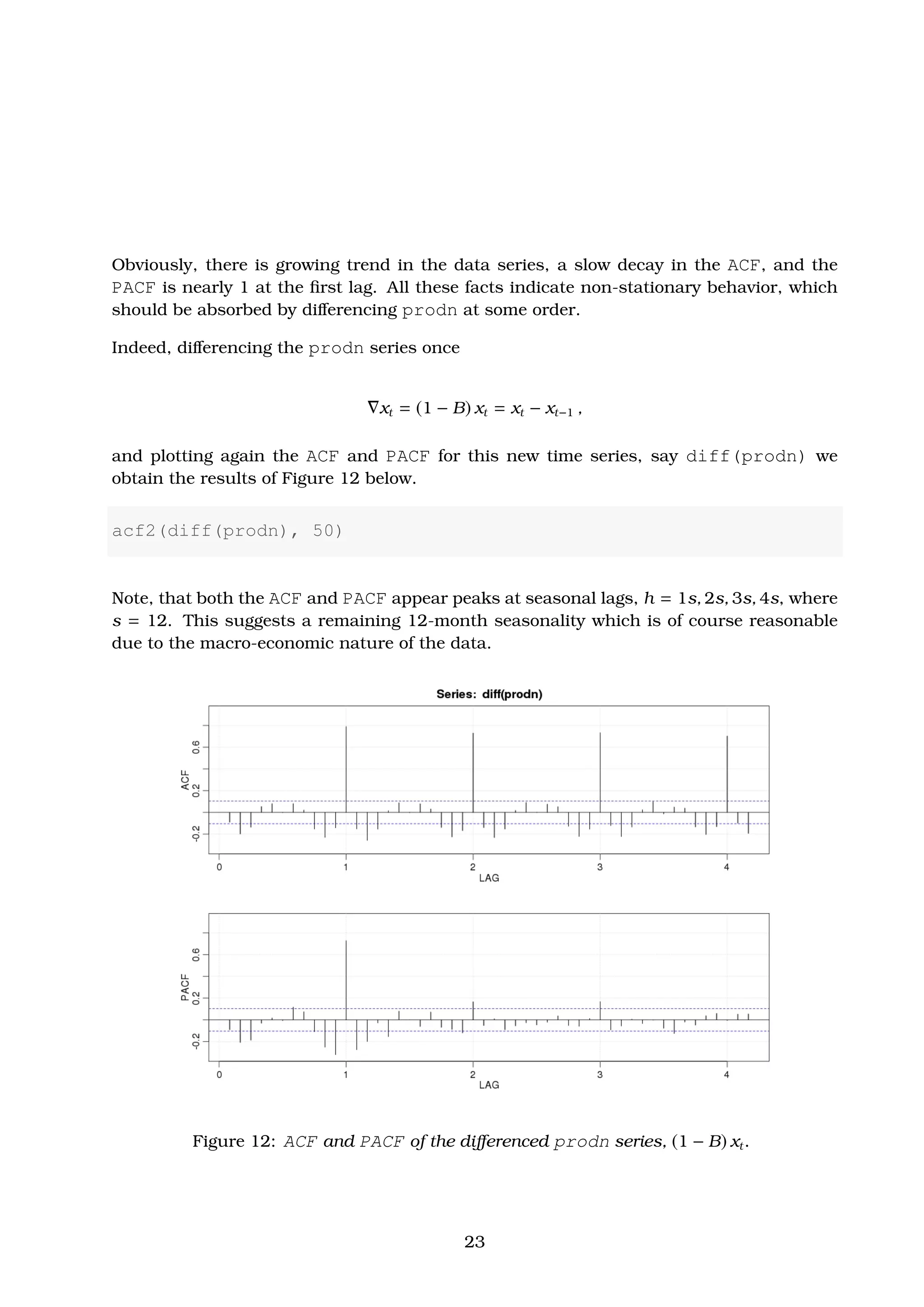
This document discusses ARIMA (autoregressive integrated moving average) models for time series forecasting. It covers the basic steps for identifying and fitting ARIMA models, including plotting the data, identifying possible AR or MA components using the autocorrelation function (ACF) and partial autocorrelation function (PACF), estimating model parameters, checking the residuals to validate the model fit, and choosing the best model. An example analyzes quarterly US GNP data to demonstrate these steps.

1. ARIMA Models [tSeriesR.2010.Ch3.Lab-3]
Theodore Grammatikopoulos∗
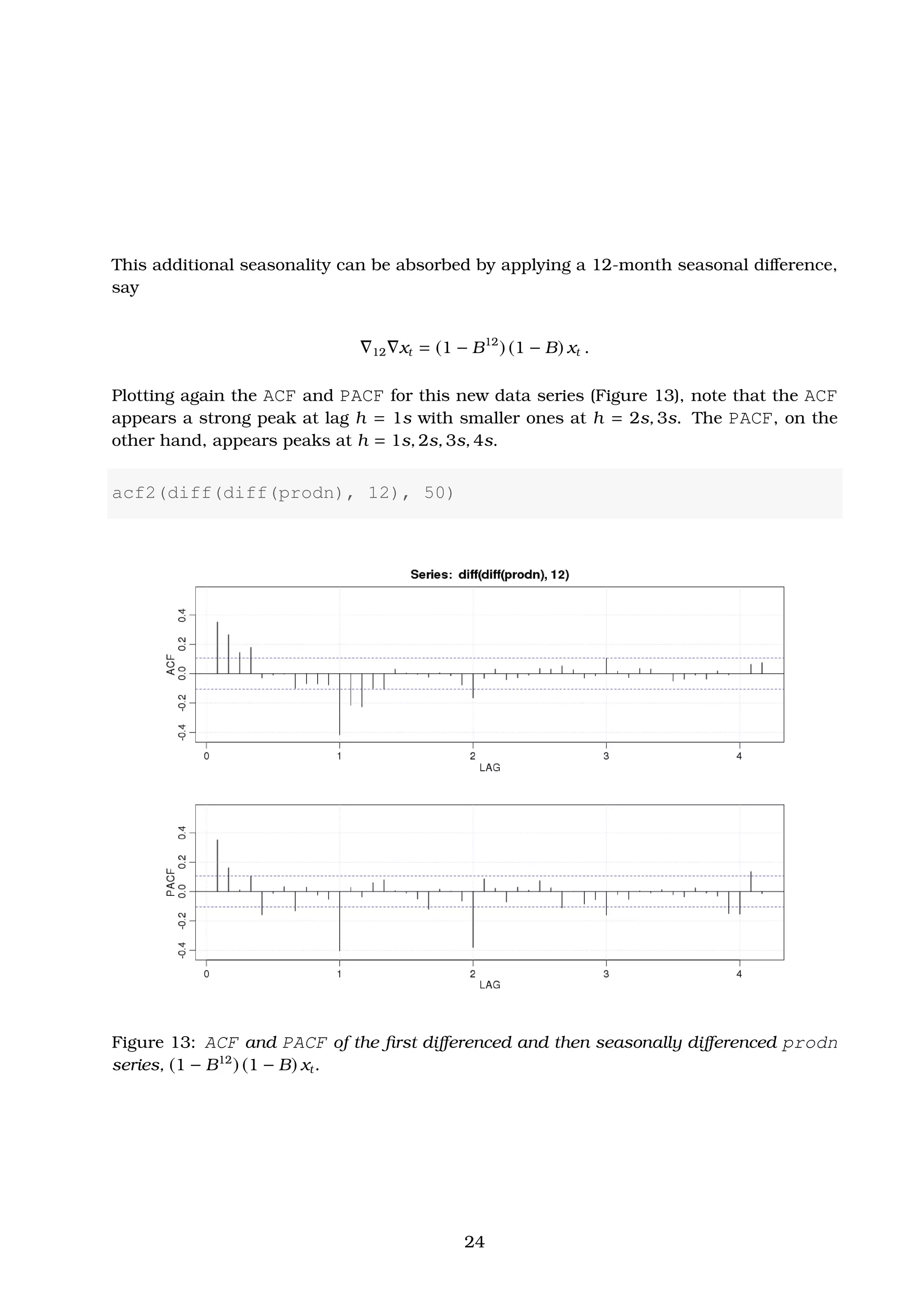
Tue 6th
Jan, 2015
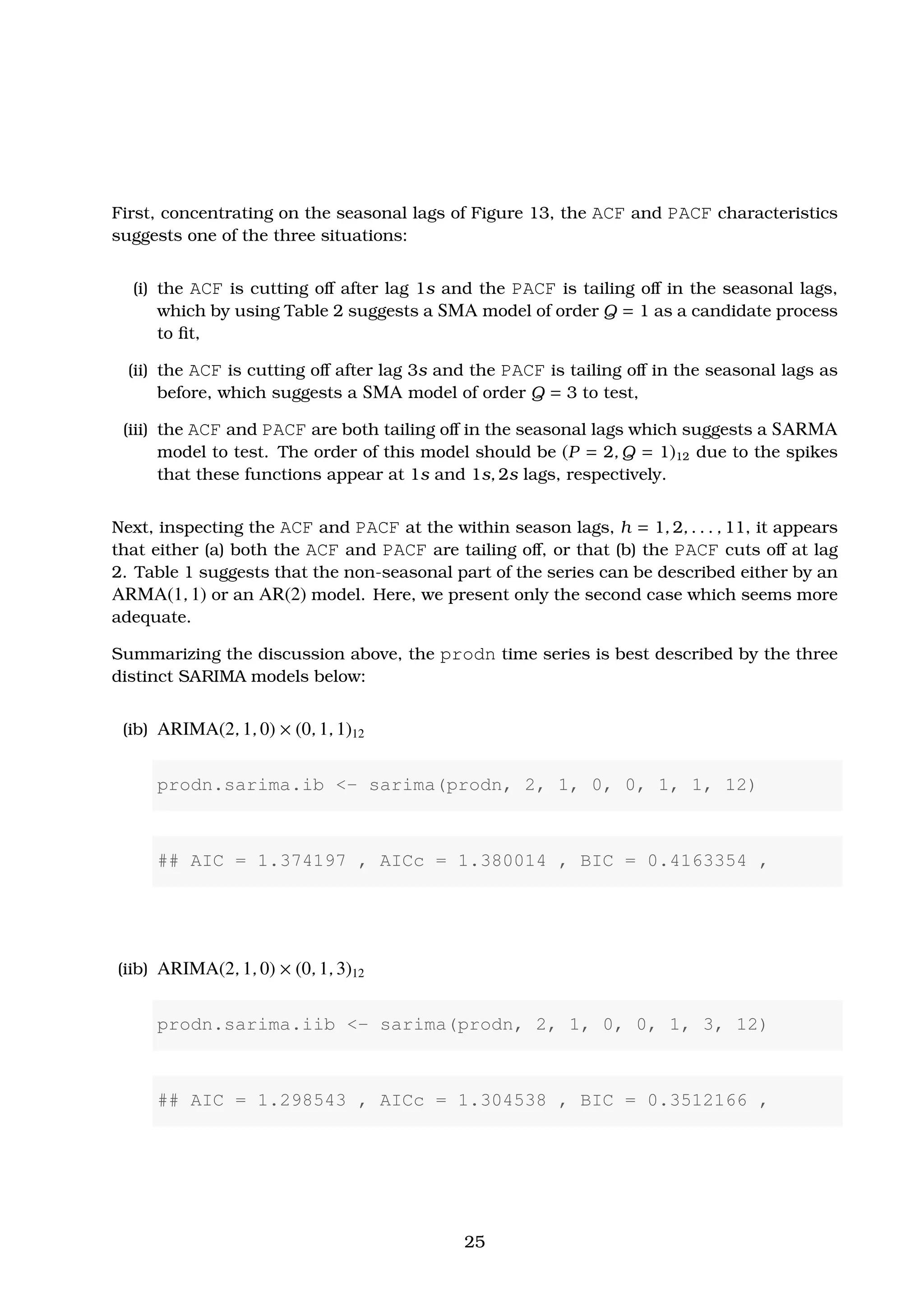
Abstract
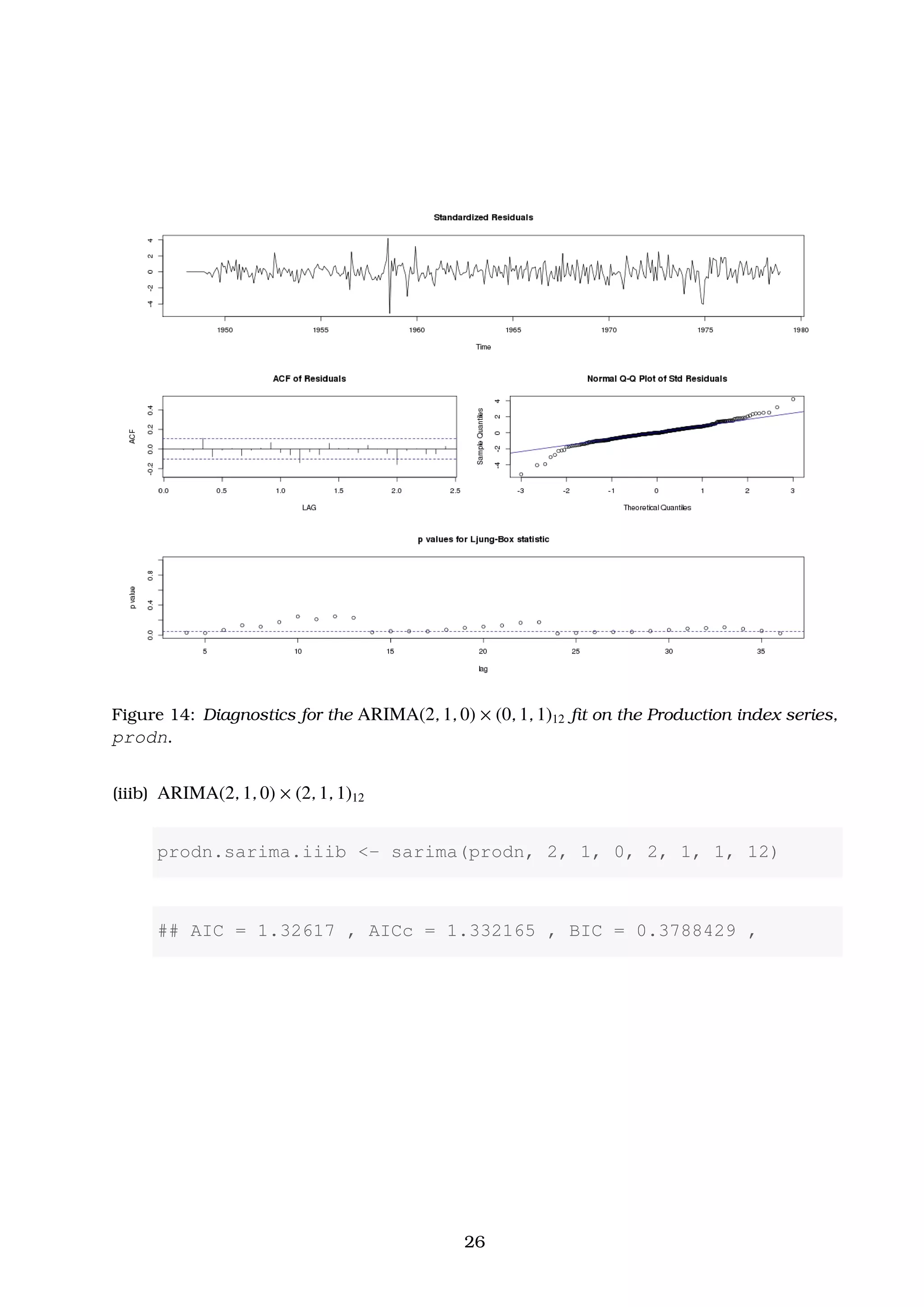
In previous articles 1 and 2, we introduced autocorrelation and cross-correlation func-
tions (ACFs and CCFs) as mathematical tools to investigate relations that may occur
within and between time series at various lags. We explained how to build linear mod-
els based on classical regression theory for exploiting the associations indicated by
the ACF or CCF. Here, we discuss time domain methods which are appropriate when
we are dealing with possibly non-stationary, shorter time series. These data series are
the rule rather than the exception in many applications, and the methods examined
here are the necessary ingredient of a successful forecasting.
Classical regression is often insufficient for explaining all of the interesting dy-
namics of a time series. For example, the ACF of the residuals of the simple linear
regression fit to the global temperature data (gtemp) reveals additional structure in
the data which is not captured by the regression (see Example 2.1 of article 2). Instead,
the correlation as a phenomenon that may be generated through lagged linear rela-
tions leads to proposing the autoregressive (AR) and autoregressive moving average
(ARMA) models. Have to also describe non-stationary processes leads to the autore-
gressive integrated moving average (ARIMA) model [Box and Jenkins, 1970]. Here we
discuss shortly the so-called Box-Jenkins method for identifying a plausible ARIMA
model, and see how it can be actually applied through practical examples. We also
apply techniques for parameter estimation and forecasting for these models.
## OTN License Agreement: Oracle Technology Network -
Developer
## Oracle Distribution of R version 3.0.1 (--) Good Sport
## Copyright (C) The R Foundation for Statistical Computing
## Platform: x86_64-unknown-linux-gnu (64-bit)
D:20150106215920+02’00’
∗
e-mail: tgrammat@gmail.com
1

2. 1 Forecasting
Example 1.1. Preliminary Analysis and Forecasting of the Recruitment Series. Here
we provide a preliminary analysis of modeling the Recruitment Series, rec, shown in Figure
2 below. We find that a second order (p = 2) autoregressive model might provide a good fit.
Then, we actually make some forecasts for a period of the next 12 months (Figure 2). Notice
how the forecast levels off quickly, whereas the prediction intervals are widening.
Solution. In rec series there are 453 months of observed recruitment ranging over 1950−
1987. In Figure 1, we plot rec’s ACF and PACF which appear to be consistent with the
behavior of an AR(2) model. This is because the ACF has cycles corresponding roughly
to a 12-month period, and the PACF has large values for h = 1, 2, being actually zero for
higher order lags. Based on Table 1, these results suggest that a second-order (p = 2)
autoregressive model might provide a good fit.
par(opar)
acf2(rec, 48) # will produce values and graphic
AR(p) MA(q) ARMA(p, q)
ACF Tails Off
Cuts Off
after lag q
Tails Off
PACF
Cuts Off
after lag p
Tails Off Tails Off
Table 1: Behavior of the ACF and PACF for ARMA Models.
Indeed, assuming that the rec series can be explained by an AR(2) model
xt = φ0 + φ1xt−1 + φ2xt−2 + wt , for t = 3, 4, . . . , 453
regr <- ar.ols(rec, order = 2, demean = FALSE, intercept = TRUE)
2

3. Figure 1: Behavior of the ACF and PACF for ARMA Models.
regr
##
## Call:
## ar.ols(x = rec, order.max = 2, demean = FALSE, intercept =
TRUE)
##
## Coefficients:
## 1 2
## 1.3541 -0.4632
##
## Intercept: 6.737 (1.111)
##
3

4. ## Order selected 2 sigma^2 estimated as 89.72
and make a forecast for the next 24 months
fore <- predict(regr, n.ahead = 24)
ts.plot(rec, fore$pred, col = 1:2, xlim = c(1980, 1990))
lines(fore$pred, type = "p", col = 2)
lines(fore$pred + fore$se, lty = "dashed", col = 4)
lines(fore$pred - fore$se, lty = "dashed", col = 4)
As shown in Figure 2 below, the forecast levels off quickly and the prediction intervals are
widening fast enough, even though in this case the forecast limits are only based on one
standard error; that is xn
n+m ± Pm
n+m.
Figure 2: Twenty-four month ahead forecast for the Recruitment series rec. The actual
data shown are from about January 1980 to September 1987, and then the forecasts plus
and minus one standard error are displayed.
4

5. 2 Estimation
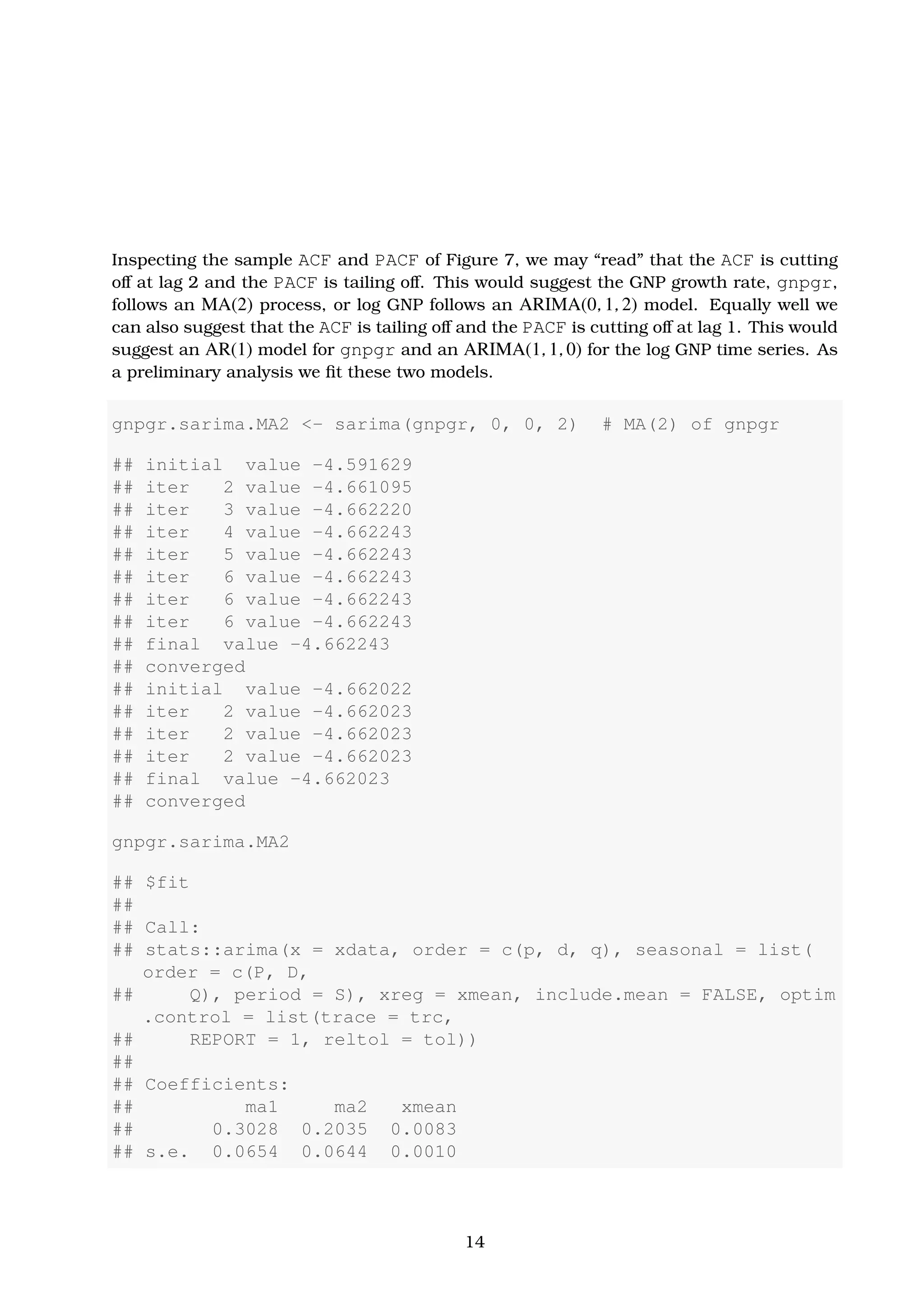
Example 2.1. Yule-Walker (YW) Estimation of the Recruitment Series (rec)
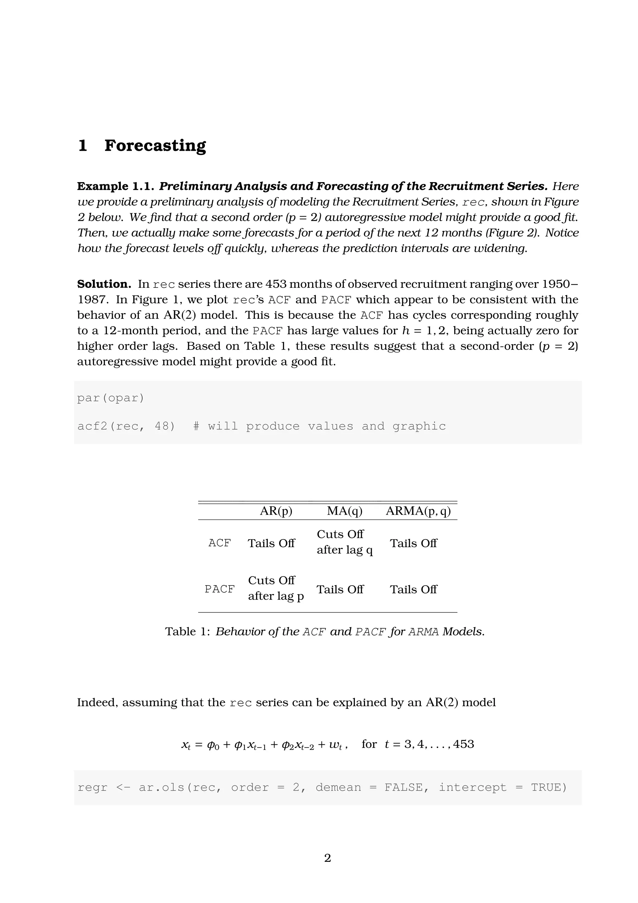
Solution. In Example 1.1 we fit an AR(2) model to the recruitment series using regression.
Here, we calculate the coefficients of the same model using Yule-Walker estimation in R.
The coefficients of the estimated model are nearly identical with the ones found in Example
1.1.
# YW Estimation of an AR(2) - rec series
rec.yw <- ar.yw(rec, order = 2)
rec.yw$x.mean # = 62.26278 (mean estimate)
## [1] 62.26278
rec.yw$ar # = 1.3315874, -.4445447 (AR parameter estimates)
## [1] 1.3315874 -0.4445447
sqrt(diag(rec.yw$asy.var.coef)) # = .04222637, .04222637 (
standard errors)
## [1] 0.04222637 0.04222637
rec.yw$var.pred # = 94.79912 (error variance estimate)
## [1] 94.79912
# 24-month ahead Forecast
rec.pr <- predict(rec.yw, n.ahead = 24)
U <- rec.pr$pred + rec.pr$se
L <- rec.pr$pred - rec.pr$se
minx <- min(rec, L)
maxx <- max(rec, U)
dev.new()
opar <- par(no.readonly = TRUE)
5

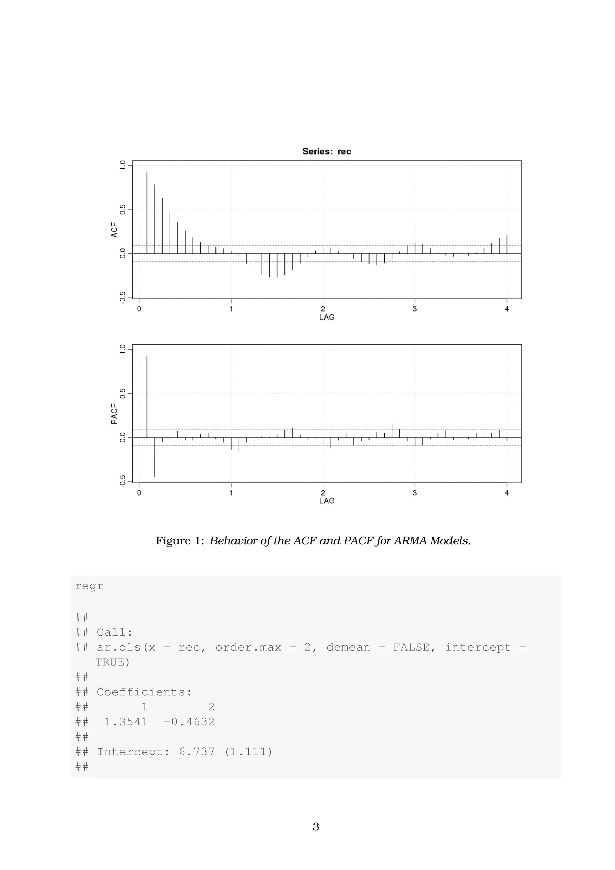
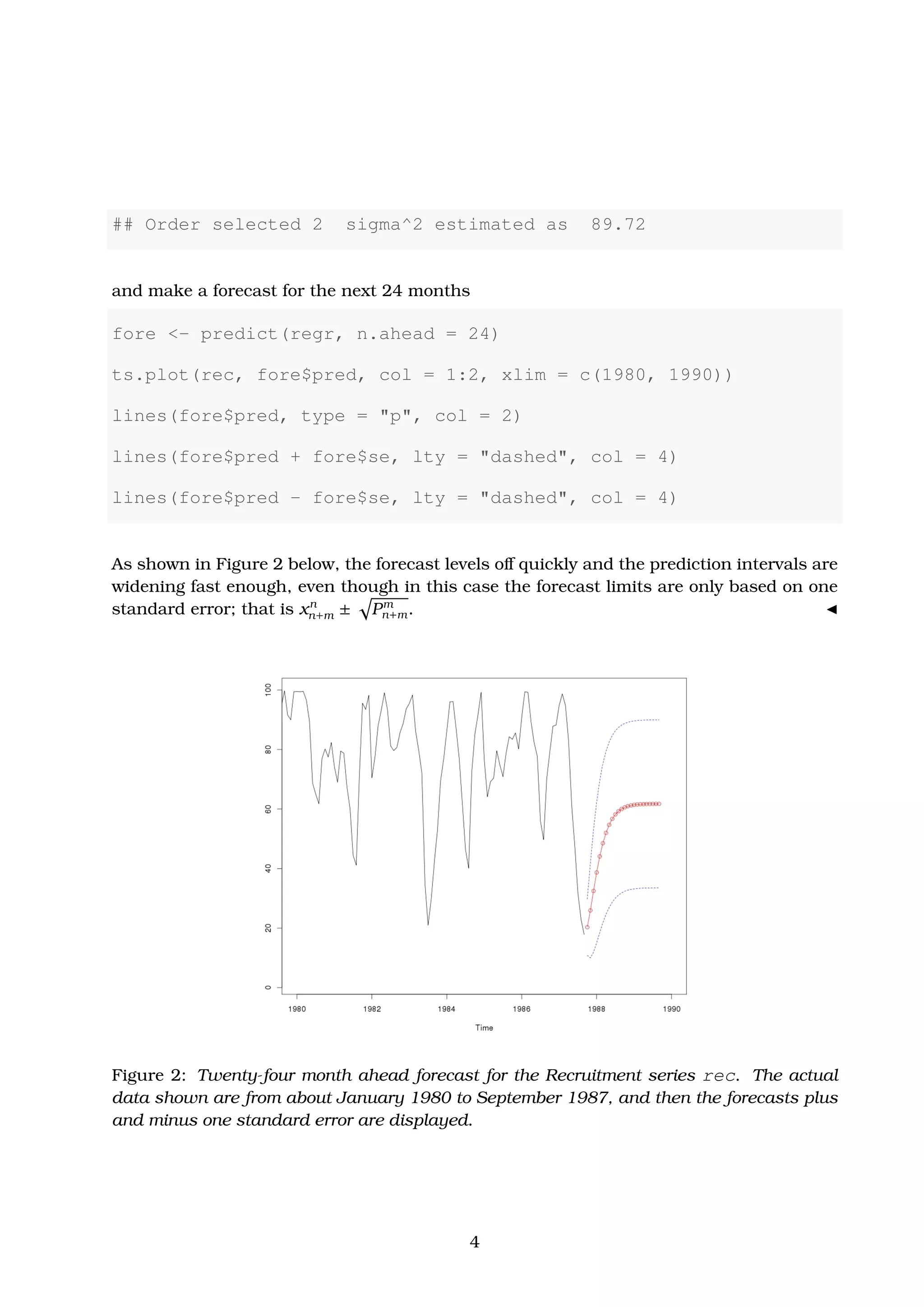
6. par(opar)
ts.plot(rec, rec.pr$pred, xlim = c(1980, 1990), ylim = c(minx,
maxx), ylab = "rec", main = "24-month ahead forecast of
Recruitment Seriesn[rec, Yule-Walker (red,blue), MLE(
green)]")
lines(rec.pr$pred, col = "red", type = "o")
lines(U, col = "blue", lty = "dashed")
lines(L, col = "blue", lty = "dashed")
Figure 3: Twenty-four month ahead forecast for the Recruitment series rec. The actual
data shown are from about January 1980 to September 1987, and then the forecasts plus
and minus one standard error are displayed. The plot has been produced by fitting an
AR(2) process using first Yule-Walker estimation (red curve with blue upper and lower
bounds) and MLE (green curves) afterwards.
6

7. Example 2.2. MLE for the Recruitment Series (rec).
Solution. Here we fit again an AR(2) model to the Recruitment time series (rec) but using
the so-called Maximum Likelihood Estimation (MLE). These results can be compared to the
results in Examples 1.1 and 2.1. Obviously, both estimation methods, YW and MLE,
produce similar forecasts for the next 24 months (Figure 3), but MLE is more accurate as
far as its error variance estimate concerns.
# MLE of an AR(2) - rec series
rec.mle <- ar.mle(rec, order = 2)
rec.mle$x.mean # = 62.26153 (mean estimate)
rec.mle$ar # = 1.3512809 -0.4612736 (AR parameter estimates)
sqrt(diag(rec.mle$asy.var.coef)) # = 0.04099159 0.04099159 (
standard errors)
rec.mle$var.pred # = 89.33597 (error variance estimate)
# 24-month ahead Forecast
rec.mle.pr <- predict(rec.mle, n.ahead = 24)
U.mle <- rec.mle.pr$pred + rec.mle.pr$se
L.mle <- rec.mle.pr$pred - rec.mle.pr$se
lines(rec.mle.pr$pred, col = "green", type = "l")
lines(U.mle, col = "green", lty = "dashed")
lines(L.mle, col = "green", lty = "dashed")
7

8. 3 Building ARIMA Models
There are a few basic steps fitting ARIMA models to time series data. These steps involve:
1. Plotting the data. First, as with any data analysis, we should construct a time plot
of the data, and inspect the graph for any anomalies. If for example, the variability of
the data series grows with time, it will be necessary to transform the data to stabilize
the variance. In such cases, the Box-Cox class of power transformations
yt =



(xλ
t − 1)/λ , λ 0
log xt , λ = 0
(1)
could be employed.
2. Transforming the data. Having recognized a suitable transformation to apply on the
data series, we continue with the exploratory data analysis to check if any additional
transformation is required.
3. Recognize possible ARIMA(p, d, q) models to test. Identify preliminary values of
the order of differencing, d, the autoregressive order, p, and the moving average
order, q.
ˆ A time plot of the data will typically suggest whether any differencing is needed.
However, be careful not to over-difference because this may introduce depen-
dence when none exists. For example, xt = wt is serially uncorrelated, but
xt = wt − wt−1 is MA(1).
ˆ A second criterion to determine if differencing is required, can be provided by the
sample ACF. In such cases, the associated polynomial has the form φ(z)(1 −z)d
and thus it includes a unit root. Therefore, the sample ACF, ρ(h), will not decay
to zero fast as h increases. Conversely, a slow decay in ρ(h) is an indication
that differencing may be needed.
ˆ Having settled a preliminary value of differencing, d, the next step is to examine
the sample ACF and PACF of d
xt. Table 1 provides a definite guide to recognize
the correct ARMA(p, q) model to test. Note, that because we are dealing with
estimates, it will not always be clear whether the sample ACF or PACF is tailing
off or cutting off. Furthermore, two models that are seemingly different may
actually be very similar. However, at this stage of model fitting we do not need
to be precise. We only need some preliminary suggested ARIMA(p, d, q) models
to estimate their parameters and finally test.
4. Parameter estimation. Having determine a preliminary set of ARIMA(p, d, q) model
we proceed with their parameter estimation. To do so we use either (a) The method
of Yule-Walker Estimation (YW), or (b) The method of Maximum Likelihood and Least
Square Estimation (MLE), which is more precise for large data samples.
8

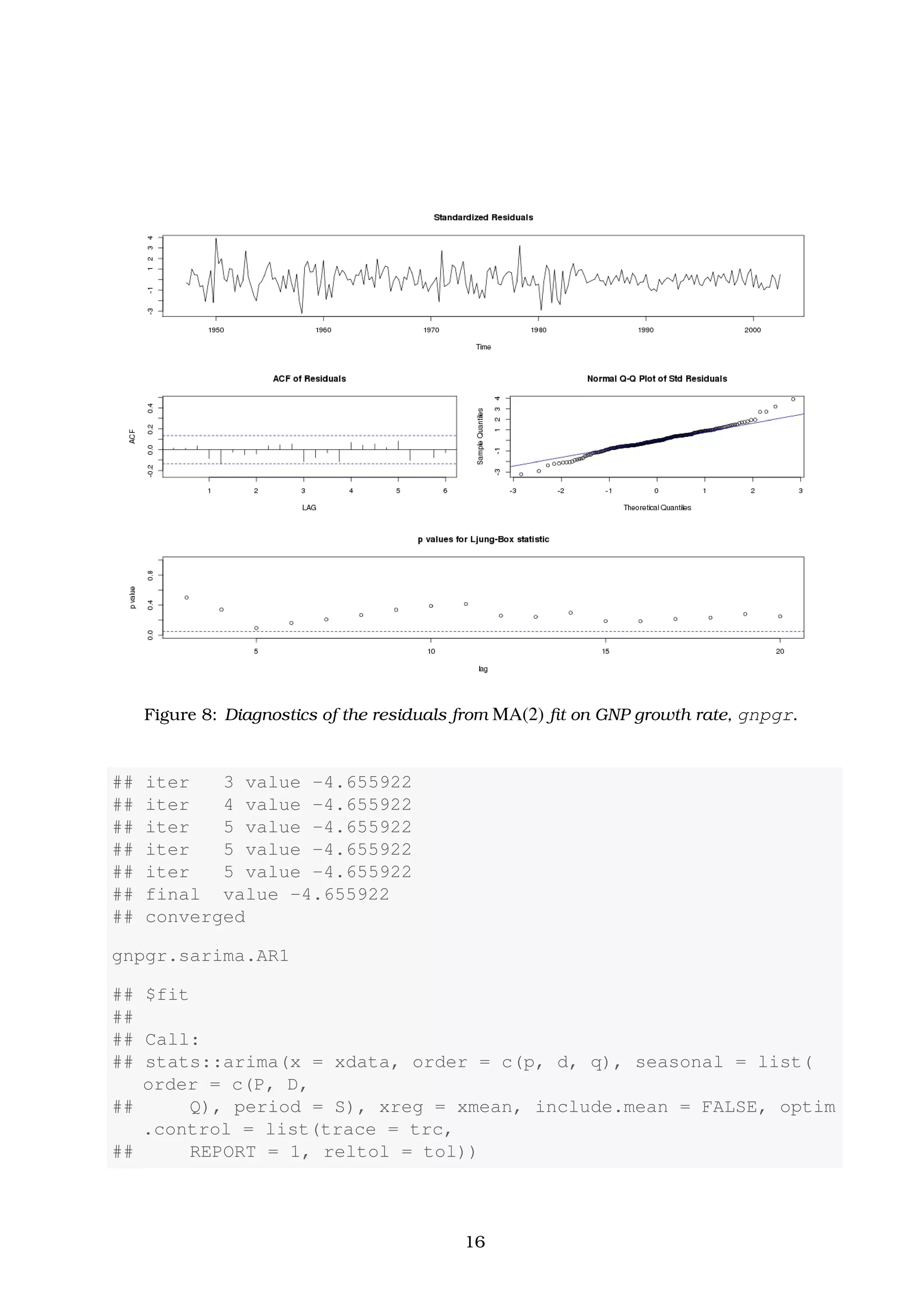
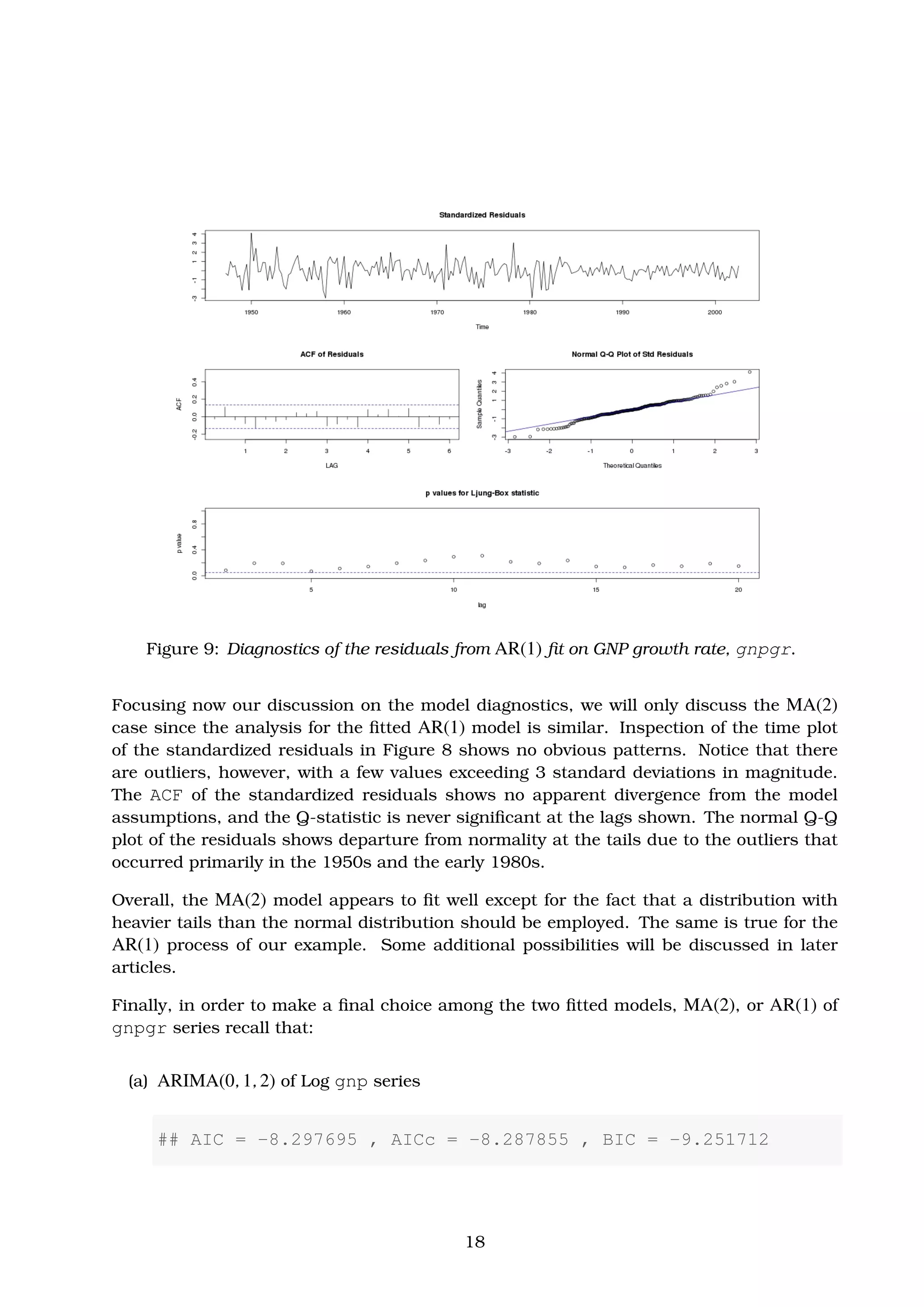
9. 5. Model diagnostics. This step includes the analysis of the residuals as well as model
comparisons.
ˆ First, we produce a time plot of the innovations (or residuals), xt − xt
t−1
, or of
the standardized innovations
et = (xt − xt
t−1
)/ (Pt
t−1
) . (2)
Here, xt
t−1
is the one-step-ahead prediction of xt (based on the fitted model) and
Pt
t−1
is the estimated one-step-ahead error variance. If the model provides a good
fit to the observational data, the standardized residuals, et, should behave as
et ∼ N(0, 1) . (3)
However, unless the time series is Gaussian, it is not enough that the residuals
are uncorrelated. For example, it is possible in the non-Gaussian case to have
an uncorrelated process for which values contiguous in time are highly depen-
dent. An important class of such models are the so-called, GARCH models.
ˆ In case that a time plot of residuals appears marginal normality a histogram
of the residuals may be extremely helpful. In addition to this, a normal prob-
ability plot or a Q-Q plot can help in identifying departures from normality.
For details of this test as well as additional tests for multivariate normality
consult [Johnson and Wichern, 2013].
ˆ Another test to search for possible departure from normality is to inspect the
sample autocorrelations of the residuals, ρe(h), for any patterns or large values.
Recall that, for a white noise sequence
ρe(h) ∼ iid N(0, 1/n) . (4)
Divergences from this expected result and beyond its expected error bounds,
±2/
√
n, suggest that the fitted model can be improved. For details consult [Box
and Pierce, 1970] and [McLeod, 1978].
ˆ A more general test takes into consideration the magnitudes of ρe(h) as a group.
For example, it may be the case that, individually, each ρe(h) is slightly less
in magnitude than the expected error bounds, 2/
√
n, but the ρe(h) as a whole
follows collectively a different statistic than the one expected by an iid N(0, 1/n)
distribution. More specifically, the statistic of interest to perform this test is
Ljung-Box-Pierce
Statistic
: Q = n(n + 2)
H
h=1
ρe
2
(h)
n − h
n→∞
−−−−→ XH−p−q . (5)
The value H in eq. (5) above is chosen somewhat arbitrarily, typically, H = 20.
Then, under the null hypothesis of model adequacy, Q
n→∞
−−−−→ XH−p−q. Thus, we
9

10. would reject the null hypothesis at level α if the value of Q exceeds the (1 − α)
quantile of X2
H−p−q distribution. For details consult [Box and Pierce, 1970],
[Ljung and Box, 1978] and [Davies et al., 1977]. The basic idea is that providing
wt describes white noise, the n ρw
2
(h), for h = 1, . . . , H, are asymptotically
independent χ2
1 random variables, which in turn means n H
h=1 ρw
2
(h) ∼ X2
H .
The loss of p + q degrees of freedom in eq. (5) is because the test involves ACF
of residuals from ARMA(p, q) model fit.
6. Model choice. In this final step of model fitting we must decide which model we will
retain for forecasting. The most popular criteria to do so are AIC, AICc and BIC.
Example 3.1. Analysis of GNP Data. Here, we consider the analysis of quarterly U.S. GNP
from 1947 to 2002, gnp, having n = 223 observations. The data are real U.S. gross national
product in billions of dollars and have been seasonally adjusted. The data were obtained
from the Federal Reserve Bank of St. Louis (http://research.stlouisfed.org) and
they are provided by the astsa package of [Shumway and Stoffer, 2013]. We are going to
make a preliminary exploratory data analysis, determine if we need to transform our data
and make a preliminary claim of possible ARIMA(p, d, q) models to fit. We will estimate
the model parameters and make a first conclusion on the performance of the produced fits.
Finally, we decide which model we will retain for forecasting and make an actual forecast.
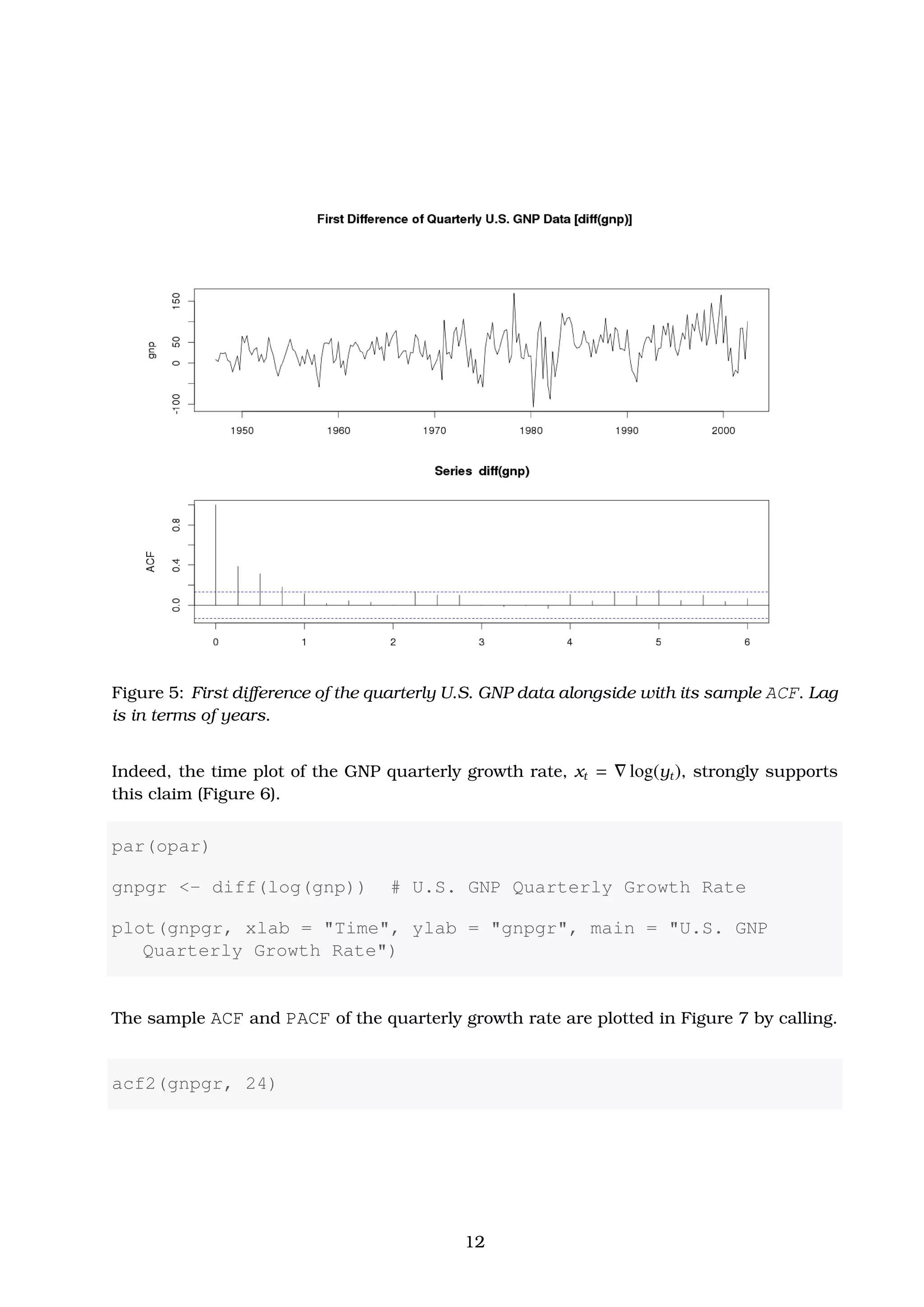
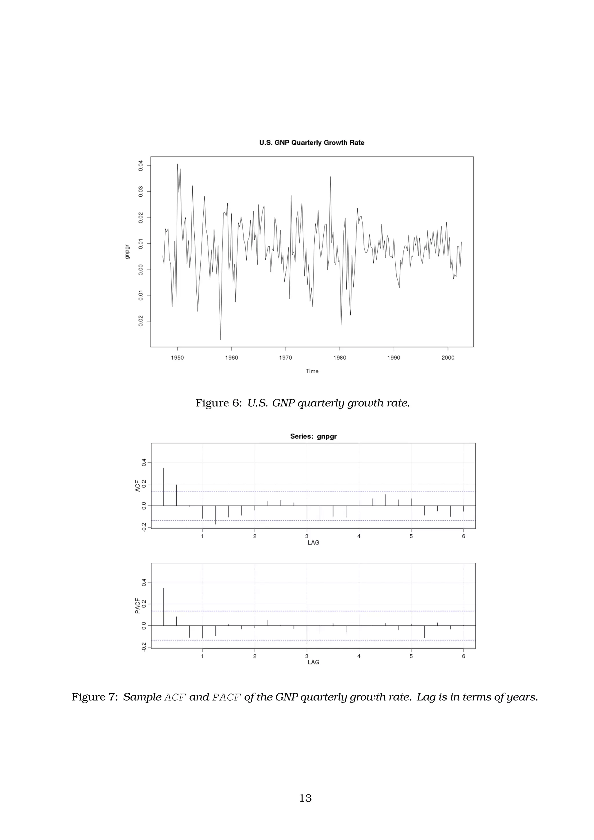
Solution. To have a first idea of the gnp data series, yt, we produce a time plot of the data
alongside with its sample ACF. As shown in Figure 4, the gnp time series appears a strong
trend of growing GNP with time, and it is not clear that the variance is also increasing.
The sample ACF, on the other hand, decay slowly with growing lag, h, indicating that we
should differ the time series first.
par(opar)
par(mfrow = c(2, 1), mar = c(3, 4.1, 4.1, 3), oma = c(0, 0, 3,
0))
plot(gnp, xlab = "Time", ylab = "gnp")
acf(gnp, 50, xlab = "Lag", ylab = "ACF") # Maximum 50 Lags
title(main = "Quarterly U.S. GNP (gnp)", outer = TRUE)
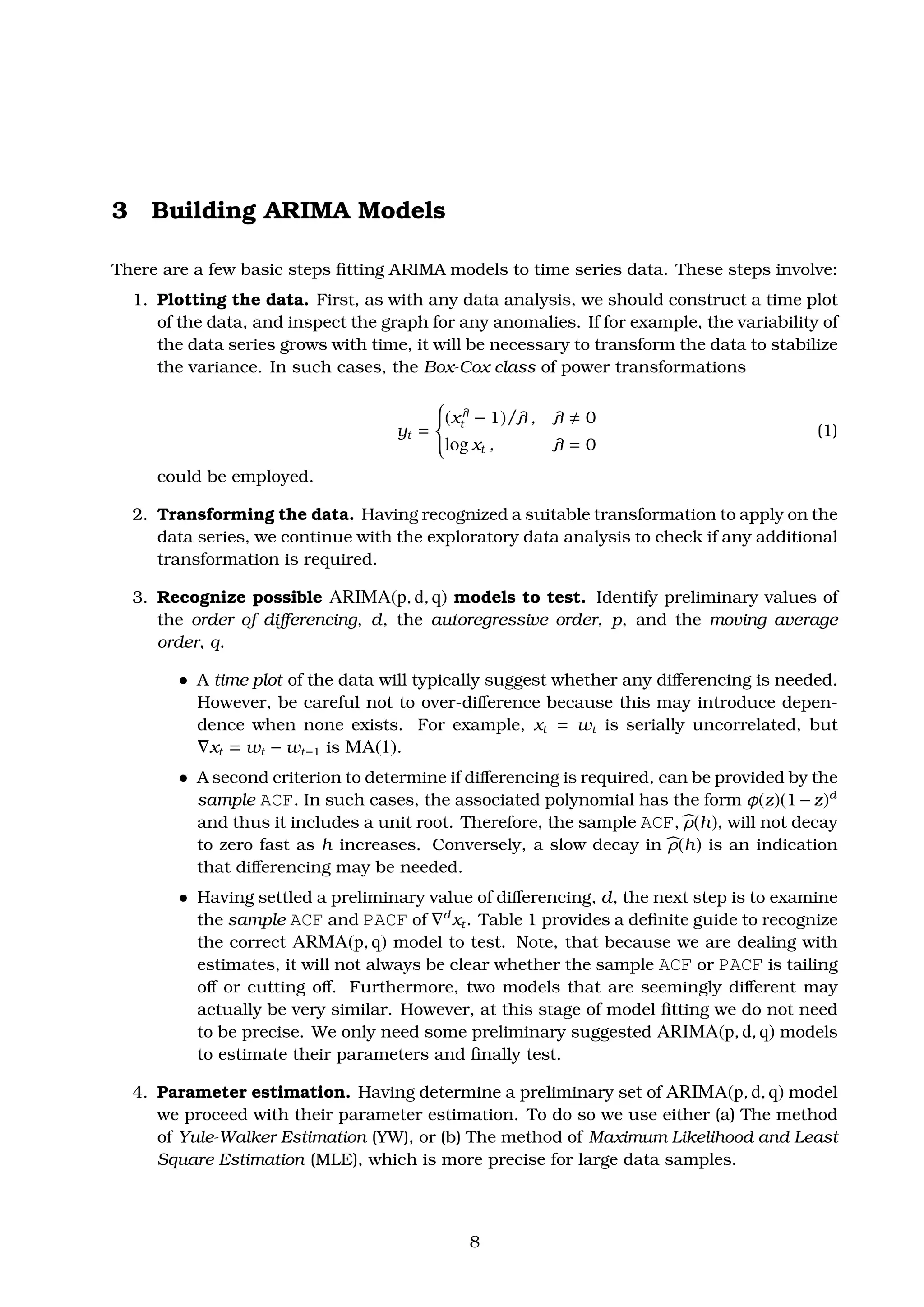
Differencing the gnp time series once and re-plotting this new data series diff(gnp), we
observe in Figure 5 that the strong growing trend has been removed and a larger variability
in the second half of the time plot has been revealed. This suggests that an additional
log-transform of the gnp data may result in a more stable process.
10

11. par(opar)
par(mfrow = c(2, 1), mar = c(3, 4.1, 4.1, 3), oma = c(0, 0, 3,
0))
plot(diff(gnp), xlab = "Time", ylab = "gnp")
acf(diff(gnp), 24, xlab = "Lag", ylab = "ACF") # Maximum 50 Lags
title(main = "First Difference of Quarterly U.S. GNP Data [diff(
gnp)]",
outer = TRUE)
Figure 4: Quarterly U.S. GNP from 1947 to 2002 alongside with its sample ACF. Lag is in
terms of years.
11

12. Figure 5: First difference of the quarterly U.S. GNP data alongside with its sample ACF. Lag
is in terms of years.
Indeed, the time plot of the GNP quarterly growth rate, xt = log(yt), strongly supports
this claim (Figure 6).
par(opar)
gnpgr <- diff(log(gnp)) # U.S. GNP Quarterly Growth Rate
plot(gnpgr, xlab = "Time", ylab = "gnpgr", main = "U.S. GNP
Quarterly Growth Rate")
The sample ACF and PACF of the quarterly growth rate are plotted in Figure 7 by calling.
acf2(gnpgr, 24)
12

13. Figure 6: U.S. GNP quarterly growth rate.
Figure 7: Sample ACF and PACF of the GNP quarterly growth rate. Lag is in terms of years.
13

14. Inspecting the sample ACF and PACF of Figure 7, we may “read” that the ACF is cutting
off at lag 2 and the PACF is tailing off. This would suggest the GNP growth rate, gnpgr,
follows an MA(2) process, or log GNP follows an ARIMA(0, 1, 2) model. Equally well we
can also suggest that the ACF is tailing off and the PACF is cutting off at lag 1. This would
suggest an AR(1) model for gnpgr and an ARIMA(1, 1, 0) for the log GNP time series. As
a preliminary analysis we fit these two models.
gnpgr.sarima.MA2 <- sarima(gnpgr, 0, 0, 2) # MA(2) of gnpgr
## initial value -4.591629
## iter 2 value -4.661095
## iter 3 value -4.662220
## iter 4 value -4.662243
## iter 5 value -4.662243
## iter 6 value -4.662243
## iter 6 value -4.662243
## iter 6 value -4.662243
## final value -4.662243
## converged
## initial value -4.662022
## iter 2 value -4.662023
## iter 2 value -4.662023
## iter 2 value -4.662023
## final value -4.662023
## converged
gnpgr.sarima.MA2
## $fit
##
## Call:
## stats::arima(x = xdata, order = c(p, d, q), seasonal = list(
order = c(P, D,
## Q), period = S), xreg = xmean, include.mean = FALSE, optim
.control = list(trace = trc,
## REPORT = 1, reltol = tol))
##
## Coefficients:
## ma1 ma2 xmean
## 0.3028 0.2035 0.0083
## s.e. 0.0654 0.0644 0.0010
14

15. ##
## sigma^2 estimated as 8.919e-05: log likelihood = 719.96, aic
= -1431.93
##
## $AIC
## [1] -8.297695
##
## $AICc
## [1] -8.287855
##
## $BIC
## [1] -9.251712
That is using MLE to fit the MA(2) model for the growth rate, xt, the estimated model is
found to be
xt = 0.0083(0.0010) + 0.3028(0.0654)wt−1 + 0.2035(0.0644)wt−2 + wt , (6)
where σw = 8.919 × 10−05
. The values in parentheses are the corresponding estimated
errors. Note, that all of the regression coefficients are significant, including the constant∗
.
In this example, not including a constant assumes the average quarterly growth rate is
zero, whereas in fact the average quarterly growth rate is about 1% (Figure 6).
The estimated AR(1) model, on the other hand, is calculated as follows.
gnpgr.sarima.AR1 <- sarima(gnpgr, 1, 0, 0) # AR(1) of gnpgr
## initial value -4.589567
## iter 2 value -4.654150
## iter 3 value -4.654150
## iter 4 value -4.654151
## iter 4 value -4.654151
## iter 4 value -4.654151
## final value -4.654151
## converged
## initial value -4.655919
## iter 2 value -4.655921
∗
Some software packages do not fit a constant in a differenced model.
15

16. Figure 8: Diagnostics of the residuals from MA(2) fit on GNP growth rate, gnpgr.
## iter 3 value -4.655922
## iter 4 value -4.655922
## iter 5 value -4.655922
## iter 5 value -4.655922
## iter 5 value -4.655922
## final value -4.655922
## converged
gnpgr.sarima.AR1
## $fit
##
## Call:
## stats::arima(x = xdata, order = c(p, d, q), seasonal = list(
order = c(P, D,
## Q), period = S), xreg = xmean, include.mean = FALSE, optim
.control = list(trace = trc,
## REPORT = 1, reltol = tol))
16

17. ##
## Coefficients:
## ar1 xmean
## 0.3467 0.0083
## s.e. 0.0627 0.0010
##
## sigma^2 estimated as 9.03e-05: log likelihood = 718.61, aic
= -1431.22
##
## $AIC
## [1] -8.294403
##
## $AICc
## [1] -8.284898
##
## $BIC
## [1] -9.263748
Thus, the AR(1) model for the growth rate, xt, is found to be
xt = 0.0083(0.0010)(1 − 0.3467) + 0.3467(0.0627)xt−1 + wt , (7)
where σw = 9.03 × 10−05
and the intercept now is 0.0083(1 − 0.3467) ≈ 0.005.
Before we discuss the produced diagnostics of these two models, we can make a first
comparison among them. They are nearly the same. This is because the fitted AR(1)
model is similar to the MA(2) one, providing that it is written in its causal form.
ARMAtoMA(ar = 0.3467, ma = 0, 10)
## [1] 3.467000e-01 1.202009e-01 4.167365e-02 1.444825e-02
## [5] 5.009210e-03 1.736693e-03 6.021115e-04 2.087520e-04
## [9] 7.237433e-05 2.509218e-05
That is the fitted AR(1) model in its causal form can be approximated by the MA(2) model
xt ≈ 0.35wt−1 + 0.12wt−2 + wt .
This process is indeed similar with the fitted MA(2) model of eq. (6).
17

18. Figure 9: Diagnostics of the residuals from AR(1) fit on GNP growth rate, gnpgr.
Focusing now our discussion on the model diagnostics, we will only discuss the MA(2)
case since the analysis for the fitted AR(1) model is similar. Inspection of the time plot
of the standardized residuals in Figure 8 shows no obvious patterns. Notice that there
are outliers, however, with a few values exceeding 3 standard deviations in magnitude.
The ACF of the standardized residuals shows no apparent divergence from the model
assumptions, and the Q-statistic is never significant at the lags shown. The normal Q-Q
plot of the residuals shows departure from normality at the tails due to the outliers that
occurred primarily in the 1950s and the early 1980s.
Overall, the MA(2) model appears to fit well except for the fact that a distribution with
heavier tails than the normal distribution should be employed. The same is true for the
AR(1) process of our example. Some additional possibilities will be discussed in later
articles.
Finally, in order to make a final choice among the two fitted models, MA(2), or AR(1) of
gnpgr series recall that:
(a) ARIMA(0, 1, 2) of Log gnp series
## AIC = -8.297695 , AICc = -8.287855 , BIC = -9.251712
18

19. (b) ARIMA(1, 1, 0) of Log gnp series
## AIC = -8.297695 , AICc = -8.287855 , BIC = -9.251712
Therefore, the AIC and AICc both prefer the MA(2) fit, whereas the BIC selects the
simpler AR(1) process. It is often the case that the BIC will select a model of smaller
order than the AIC or AICc. Pure autoregressive models, on the other hand, are easier to
work with. Thus, it is not unreasonable to finally retain the AR(1) fit to make forecasts.
4 Multiplicative Seasonal ARIMA Models
In this section, we discuss several modifications made to the ARIMA model to consider for
seasonal and non-stationary behavior of various more realistic processes. More specifi-
cally, the natural variability of many physical, biological, and economic processes tends
to match with seasonal fluctuations. For example, with monthly economic data, there is
a strong yearly component occurring at lags that are multiples of s = 12. Other economic
data which are aggregated at a quarterly basis of fiscal year exhibits a s = 4 seasonality.
Definition 4.1. Given the seasonal autoregressive operator, and the seasonal moving
average operator of orders P and Q, with seasonal period s, as defined below
Seasonal
AR operator
: ΦP (Bs
) = 1 − Φ1Bs
− Φ2B2s
− · · · − ΦP BPs
(8)
Seasonal
MA operator
: ΘQ(Bs
) = 1 − Θ1Bs
− Θ2B2s
− · · · − ΘQBPs
(9)
the pure seasonal autoregressive moving average model, ARMA(P, Q)s, takes the form
SARMA models : ΦP (Bs
)xt = ΘQ(Bs
)wt . (10)
Of course, ACF and PACF functions have analogous extensions in the seasonal models
paradigm. Table 2 summarizes the expected behavior of the ACF and the PACF in this
case, and it can be used as an initial diagnostic guide to recognize possible SARMA models
to fit.
19

20. AR(P)s MA(Q)s ARMA(P, Q)s
ACF*
Tails Off at lags ks
k = 1, 2, . . .
Cuts Off after
lag Qs
Tails Off at
lags ks
PACF*
Cuts Off after
lag Ps
Tails Off at lags ks
k = 1, 2, . . .
Tails Off at
lags ks
Table 2: Behavior of the ACF and PACF for SARMA Models. The values at non-seasonal
lags h ks, for k = 1, 2, . . . , are zero.
A more general class of models is the so-called multiplicative seasonal autoregressive
and moving average models, denoted by ARMA(p, q) × (P, Q)s and defined by
Multiplicative
SARMA models
: ΦP (Bs
)φ(B)xt = ΘQ(Bs
)θ(B)wt . (11)
Table 2 provides a rough guide of the indicated form of the model fit, but it is not strictly
true in this case. In fitting such models, focusing on the SARMA components first gener-
ally leads to more satisfactory results.
Another case of seasonality trend is the so-called seasonal non-stationarity. This occurs
when a process is nearly periodic in the season and it can be expressed as
xt = St + wt .
Here, St is a seasonal component that varies slowly, say, from one year to the next,
according to a random walk
St = St−12 + ut ,
and wt, ut are white noise processes, as usual. In such cases we should first absorb the
seasonal component by applying the so-called seasonal differencing, and then try to figure
out what a possible SARMA or ARIMA model might be.
Incorporating these ideas into a more general model leads to the definition of the so-called
SARIMA models.
Definition 4.2. The general form of a multiplicative seasonal autoregressive inte-
grated moving average model, or SARIMA model is given by
Multiplicative
SARIMA models
: ΦP (Bs
) φ(B) D
s
d
xt = δ + ΘQ(Bs
) θ(B) wt , (12)
20

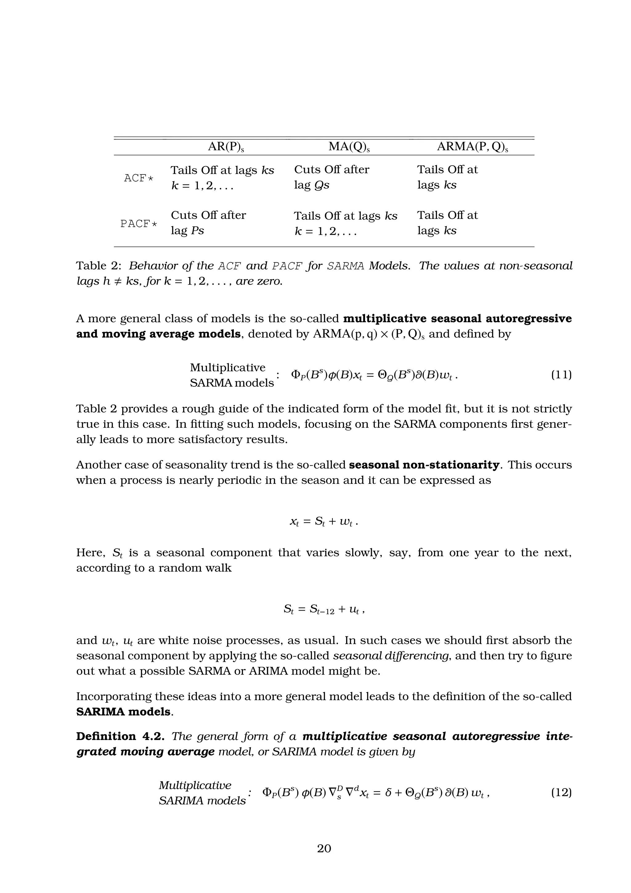
21. where wt is a Gaussian white noise process, i.e. wt ∼ iid N(0, 1). This general model is
denoted as ARIMA(p, d, q) × (P, D, Q)s.
Building SARIMA Models
Selecting the appropriate SARIMA model for a given set of data is not an easy task, but a
rough description of how doing so is the following:
1. We determine the difference (seasonal or ordinary) operators (if any) that produce a
roughly stationary series.
2. We evaluate the ACF and PACF functions of the remaining stationary data series
and using the general properties of Tables 1 and 2, we determine a preliminary set
of ARMA/SARMA models to test.
3. Given this preliminary set of ARIMA(p, d, q) × (P, D, Q)s models we proceed with their
parameter estimation. To do so we use either (a) the method of Yule-Walker Esti-
mation (YW) or (b) the method of Maximum Likelihood and Least Square Estimation
(MLE), which is more precise for large data samples.
4. Then, by using the same criteria mentioned in Section 3 (see “Model diagnostics”),
we can judge whether these models are satisfactory enough to further consider.
5. Finally, we decide which model will retain for forecasting based on their AIC, AICc
and/or BIC statistics.
Example 4.1. The Federal Reserve Board Production Index. Given the monthly time
series of “Federal Reserve Board Production Index”, prodn, which is provided by the astsa
package of [Shumway and Stoffer, 2013] and includes the monthly values of the index for
the period 1948-1978, we now fit a preliminary set of SARIMA models and finally select the
best one to make a forecast for the next 12 months.
Solution. First we provide a time plot of the prodn time series (Figure 10). In Figure 11
we also plot the ACF and PACF functions for this time series.
par(opar)
plot(prodn, main = "Monthly Federal Reserve Board Production
Indexn[prodn{astsa}, 1948-1978]")
par(opar)
acf2(prodn, 50)
21

22. Figure 10: Monthly values of the “Federal Reserve Board Production Index”, [prodn, 1948 -
1978]
Figure 11: ACF and PACF of the prodn series.
22

23. Obviously, there is growing trend in the data series, a slow decay in the ACF, and the
PACF is nearly 1 at the first lag. All these facts indicate non-stationary behavior, which
should be absorbed by differencing prodn at some order.
Indeed, differencing the prodn series once
xt = (1 − B) xt = xt − xt−1 ,
and plotting again the ACF and PACF for this new time series, say diff(prodn) we
obtain the results of Figure 12 below.
acf2(diff(prodn), 50)
Note, that both the ACF and PACF appear peaks at seasonal lags, h = 1s, 2s, 3s, 4s, where
s = 12. This suggests a remaining 12-month seasonality which is of course reasonable
due to the macro-economic nature of the data.
Figure 12: ACF and PACF of the differenced prodn series, (1 − B) xt.
23

24. This additional seasonality can be absorbed by applying a 12-month seasonal difference,
say
12 xt = (1 − B12
) (1 − B) xt .
Plotting again the ACF and PACF for this new data series (Figure 13), note that the ACF
appears a strong peak at lag h = 1s with smaller ones at h = 2s, 3s. The PACF, on the
other hand, appears peaks at h = 1s, 2s, 3s, 4s.
acf2(diff(diff(prodn), 12), 50)
Figure 13: ACF and PACF of the first differenced and then seasonally differenced prodn
series, (1 − B12
) (1 − B) xt.
24

25. First, concentrating on the seasonal lags of Figure 13, the ACF and PACF characteristics
suggests one of the three situations:
(i) the ACF is cutting off after lag 1s and the PACF is tailing off in the seasonal lags,
which by using Table 2 suggests a SMA model of order Q = 1 as a candidate process
to fit,
(ii) the ACF is cutting off after lag 3s and the PACF is tailing off in the seasonal lags as
before, which suggests a SMA model of order Q = 3 to test,
(iii) the ACF and PACF are both tailing off in the seasonal lags which suggests a SARMA
model to test. The order of this model should be (P = 2, Q = 1)12 due to the spikes
that these functions appear at 1s and 1s, 2s lags, respectively.
Next, inspecting the ACF and PACF at the within season lags, h = 1, 2, . . . , 11, it appears
that either (a) both the ACF and PACF are tailing off, or that (b) the PACF cuts off at lag
2. Table 1 suggests that the non-seasonal part of the series can be described either by an
ARMA(1, 1) or an AR(2) model. Here, we present only the second case which seems more
adequate.
Summarizing the discussion above, the prodn time series is best described by the three
distinct SARIMA models below:
(ib) ARIMA(2, 1, 0) × (0, 1, 1)12
prodn.sarima.ib <- sarima(prodn, 2, 1, 0, 0, 1, 1, 12)
## AIC = 1.374197 , AICc = 1.380014 , BIC = 0.4163354 ,
(iib) ARIMA(2, 1, 0) × (0, 1, 3)12
prodn.sarima.iib <- sarima(prodn, 2, 1, 0, 0, 1, 3, 12)
## AIC = 1.298543 , AICc = 1.304538 , BIC = 0.3512166 ,
25

26. Figure 14: Diagnostics for the ARIMA(2, 1, 0) × (0, 1, 1)12 fit on the Production index series,
prodn.
(iiib) ARIMA(2, 1, 0) × (2, 1, 1)12
prodn.sarima.iiib <- sarima(prodn, 2, 1, 0, 2, 1, 1, 12)
## AIC = 1.32617 , AICc = 1.332165 , BIC = 0.3788429 ,
26

27. Figure 15: Diagnostics for the ARIMA(2, 1, 0) × (0, 1, 3)12 fit on the Production index series,
prodn.
Judging from the diagnostics of these three models (Figures 14-16), we can easily conclude
that all of them fits well with the prodn time series, but the preferred model in terms of
the AIC, AICc and BIC statistics is the second one, (iib) ARIMA(2, 1, 0) × (0, 1, 3)12. The
fitted model in this case is:
prodn.sarima.iib
## $fit
##
## Call:
## stats::arima(x = xdata, order = c(p, d, q), seasonal = list(
order = c(P, D,
## Q), period = S), include.mean = !no.constant, optim.
control = list(trace = trc,
## REPORT = 1, reltol = tol))
##
## Coefficients:
27

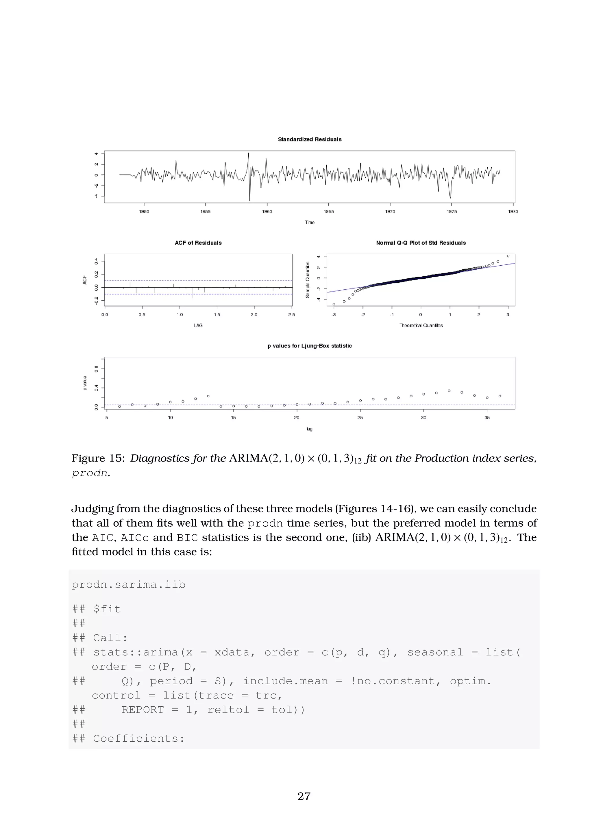
28. Figure 16: Diagnostics for the ARIMA(2, 1, 0) × (2, 1, 1)12 fit on the Production index series,
prodn.
## ar1 ar2 sma1 sma2 sma3
## 0.3038 0.1077 -0.7393 -0.1445 0.2815
## s.e. 0.0526 0.0538 0.0539 0.0653 0.0526
##
## sigma^2 estimated as 1.312: log likelihood = -563.98, aic =
1139.97
##
## $AIC
## [1] 1.298543
##
## $AICc
## [1] 1.304538
##
## $BIC
## [1] 0.3512166
28

29. or in operator form
1 − 0.3038(0.0526) B − 0.1077(0.0538) B2
12 xt =
= 1 − 0.7393(0.0539) B12
− 0.1445(0.0653) B24
+ 0.2815(0.0526) B36
wt ,
with σ2
w = 1.312.
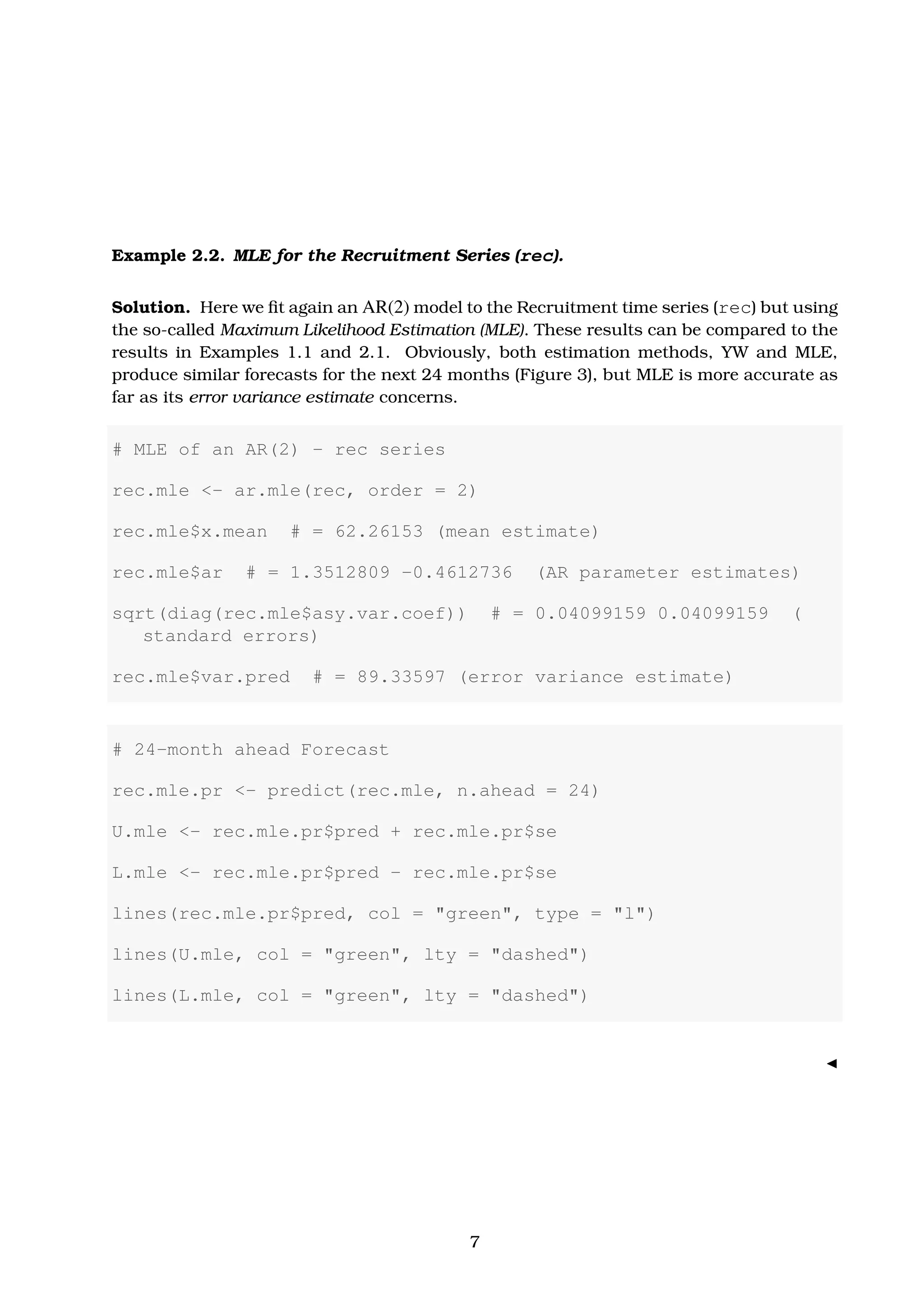
Finally, we actually make forecasts for the next 12 months using this fitted model, i.e.
(iib) ARIMA(2, 1, 0) × (0, 1, 3)12. These are shown in Figure 17 below.
prodn.sarima.iib.fore <- sarima.for(prodn, 12, 2, 1, 0, 0, 1,
3, 12) # 12-month forecast
title(main = "Federal Reserve Board Production IndexnForecasts
and Error Bound Limits [prodn{astsa}, 1948-1978]",
outer = FALSE)
Figure 17: Forecasts and error bounds for the “Federal Reserve Board Production Index”,
prodn series, based on ARIMA(2, 1, 0) × (0, 1, 3)12 fitted model [case (iib)].
29

30. References
[Box and Pierce, 1970] Box, G. and Pierce, D. (1970). Distributions of residual auto-
correlations in autoregressive integrated moving average models. J. Am. Stat. Assoc.,
72:397–402.
[Box and Jenkins, 1970] Box, G. E. P. and Jenkins, G. M. (1970). Time Series Analysis
Forecasting and Control. Holden-Day, San Francisco.
[Davies et al., 1977] Davies, N., Triggs, C., and Newbold, P. (1977). Significance levels of
the box-pierce portmanteau statistic in finite samples. Biometrica, 64:517–522.
[Johnson and Wichern, 2013] Johnson, R. A. and Wichern, D. W. (2013). Applied Multi-
variate Statistical Analysis. Pearson, 6th ed. 2013 edition.
[Ljung and Box, 1978] Ljung, L. and Box, G. E. P. (1978). On a measure of lack of fit in a
time series. Biometrica, 65:297–303.
[McLeod, 1978] McLeod, A. (1978). On the distribution of residual autocorrelations in
box-jenkins models. J. R. Stat. Soc., B(40):296–302.
[Shumway and Stoffer, 2013] Shumway, R. H. and Stoffer, D. S. (2013). Time Series Anal-
ysis and Its Applications: With R Examples (Springer Texts in Statistics). Springer,
softcover reprint of hardcover 3rd ed. 2011 edition.
30