Machine-learning models are behind many recent technological advances, including high-accuracy translations of the text and self-driving cars. They are also increasingly used by researchers to help in solving physics problems, like Finding new phases of matter, Detecting interesting outliers in data from high-energy physics experiments, Founding astronomical objects are known as gravitational lenses in maps of the night sky etc. The rudimentary algorithm that every Machine Learning enthusiast starts with is a linear regression algorithm. In statistics, linear regression is a linear approach to modelling the relationship between a scalar response (or dependent variable) and one or more explanatory variables (or independent variables). Linear regression analysis (least squares) is used in a physics lab to prepare the computer-aided report and to fit data. In this article, the application is made to experiment: 'DETERMINATION OF DIELECTRIC CONSTANT OF NON-CONDUCTING LIQUIDS'. The entire computation is made through Python 3.6 programming language in this article.

1. Linear Regression
Anirban Majumdar
June 21, 2020
Abstract
Machine-learning models are behind many recent technological ad-
vances, including high-accuracy translations of text and self-driving cars.
They are also increasingly used by researchers to help in solving physics
problems, like finding new phases of matter, detecting interesting outliers
in data from high-energy physics experiments, founding astronomical ob-
jects known as gravitational lenses in maps of the night sky etc. The rudi-
mentary algorithm that every Machine Learning enthusiast starts with is
a linear regression algorithm. In statistics, linear regression is a linear
approach to modeling the relationship between a scalar response (or de-
pendent variable) and one or more explanatory variables (or independent
variables). Linear regression analysis (least squares) is used in physics lab
in order to computer-aided analysis and to fit datas. In this article ap-
plication is made to experiment: ’DETERMINATION OF DIELECTRIC
CONSTANT OF NON-CONDUCTING LIQUIDS’. The entire computa-
tion is made through Python 3.6 programming language in this article.
1

2. 1 Theory of Linear Regression
Figure 1:
The blue stars are representing the training data points (xi, yi) and green star is the testing data point and the
red straight line is the fitted line (Getting by Least Square Approximation process). And ± i are respectively
positive and negative errors.
Let us consider that in an experiment we have measured 5 y for 5 different x (i.e.
5 blue stars). So now the objective is to predict what would be the value of y
for a different x for which we did not do the experiment explicitly. So, now one
simplest way is to draw a line through this 5 given points and once line is drawn
we can pickup any value of x, and just from the graph we can read out the value
of y corresponding to that x. Now that approach is very easy to implement.
But the main problem is there can be infinitely many curves through some finite
numbers of given data points. So now how to be know whether our line that we
have drawn is correct or not? For that we need testing data sets (indicated by
green star in the Figure- 1). Now that line is more applicable which is in close
enough to the testing data sets. Now this fitted line can be a curve line or a
straight line according to its distribution functions. In this section we will study
how a straight line can be fitted with some given data sets. The process is well
known as Linear Regression. In statistics, linear regression is a linear approach
to modeling the relationship between a scalar response (or dependent variable)
and one or more explanatory variables (or independent variables). Linear re-
gression analysis is used in physics lab in order to computer-aided analysis and
to fit datas.
Let us consider that the equation of the best fitted straight line will be y = mx+c
2

3. for some given data points (xi, yi). Now our objective is to find the value of m
and c for which the straight line will be best fitted for the given training and
testing data sets.
For this we will follow least square approximation method. According to this
theory the straight line, that minimizes the sum of the squared distances (devi-
ations) from the line to each observation (which is called error and denoted by
i for the ith
observation point), will be the best fitted straight line.
Now,
i = yi − mxi − c (1)
It should be noticed that the error of equation (1) can be positive or negative
for different given data points. But the errors should always be additive. So,
we will calculate the square of each error before adding them.
So, the total error is
E =
i
i
2
⇒ E =
i
(yi − mxi − c)
2
(2)
Now to minimize E we have the following conditions.
∂E
∂m
= 0 (3)
∂2
E
∂m2
> 0
∂E
∂c
= 0 (4)
∂2
E
∂c2
> 0
So, according to equation (4)-
−2
i
(yi − mxi − c) = 0
⇒
i
(yi − mxi − c) = 0
⇒
i
yi − m
i
xi − cn = 0
⇒ c = i yi − m i xi
n
(5)
3

4. where n is the total number of given data points
Now according to equation (3) and (5)-
−2
i
xi yi − mxi − i yi − m i xi
n
= 0
⇒ m =
n i xiyi − i xi i yi
n i xi
2 − ( i xi)
2 (6)
2 Python Programming for implementation of
Linear Regression
2.1 The Physics Problem- EXPERIMENTALLY DETER-
MINATION OF DIELECTRIC CONSTANT OF LIQ-
UIDS
Application for Linear Regression is made to experiment: ’DETERMINATION
OF DIELECTRIC CONSTANT OF LIQUIDS’.
Dielectric or electrical insulating materials are the substances in which elec-
trostatic field can persist for long times. When a dielectric is placed between
the plates of a capacitor and the capacitor is charged, the electric field between
the plates polarizes the molecules of the dielectric. This produces concentration
of charge on its surface that creates an electric field which is anti parallel to
the original field (which has polarized the dielectric). This reduces the electric
potential difference between the plates. Considered in reverse, this means that,
with a dielectric between the plates of a capacitor, it can hold a larger charge.
The extent of this effect depends on the dipole polarizability of molecules of
the dielectric, which in turn determines the dielectric constant of the material.
The method for determination of dielectric constants of liquids consists in the
successive measurement of capacitance, first in a vacuum, and then when the
capacitor is immersed in the liquid under investigation. A cylindrical capacitor
has been used for liquid samples.
4

5. Figure 2:
Dielectric measurement setup for non conducting liquids.
The capacitance per unit length of a long cylindrical capacitor immersed in
a medium of dielectric constant k is given by
C = k
2π 0
ln r2
r1
(Where 0 is free space permittivity, r1 is external radius of inner cylinder and r2 is internal radius of outer cylinder.)
In actual practice, there are errors due to stray capacitances (Cs) at the ends
of the cylinders and the leads. In any accurate measurement, it is necessary to
eliminate these. It has been done in the following way:
Consider a cylindrical capacitor of length L filled to a height h < L with a
liquid of dielectric constant k. Its total capacitance is given by-
C =
2π 0
ln r2
r1
[kh + 1 · (L − h)] + Cs
⇒ C =
2π 0
ln r2
r1
(k − 1) h +
2π 0L
ln r2
r1
+ Cs
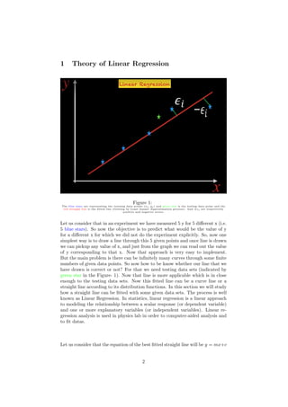
So, the above equation shows that the measured capacity C is a linear function
of h (the height upto which the liquid is filled in the capacitor). If we vary the
liquid height h, and measure it, together with the corresponding capacitance C,
the plot of the data should be a straight line. The slope of this equation is given
by-
m =
2π 0
ln r2
r1
(k − 1)
⇒ k =
m ln r2
r1
2π 0
+ 1
From the above equation we can determine k for known values of r1 and r2.
5

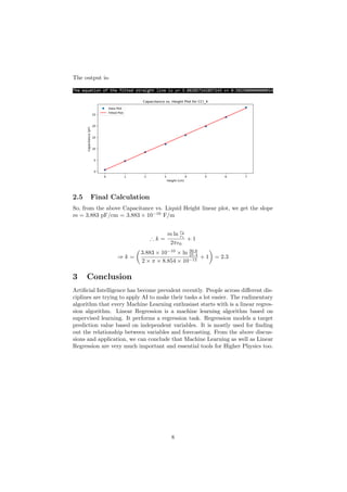
6. 2.2 Experimental Results
Liquid Sample CCl4
External radius of inner cylinder 25.4mm
Internal radius of outer cylinder 30.6mm
Liquid Height (cm) Capacitance (pF)
0.0 0.70
1.0 4.54
2.0 8.48
3.0 11.98
4.0 15.95
5.0 19.78
6.0 23.88
7.0 28.07
2.3 Fitting of Datas Using basic Linear Regression Theory
Python Coding-
import matplotlib.pyplot as plt
import numpy as np
from math import *
X=np.array([0.0,1.0,2.0,3.0,4.0,5.0,6.0,7.0])
Y=np.array([0.7,4.54 ,8.48 ,11.98 ,15.95 ,19.78 ,23.88 ,28.07])
n=X.size
sop=0
x=0
y=0
x2=0
for i in range (n):
sop=sop+(X[i]*Y[i])
x=x+X[i]
y=y+Y[i]
x2=x2+(X[i]) ** 2
m=((n*sop)-(x*y))/float ((n*x2)-(x) ** 2)
c=((y)-(m*x))/float(n)
M=np.full(n,m)
C=np.full(n,c)
Y_avg=M*X+C
print("The equation of the fitted straight line is y=",m,"x+",c)
plt.plot(X,Y,’o’)
plt.plot(X, Y_avg , color=’red ’)
plt.xlabel(’Height (cm)’)
plt.ylabel(’Capacitance (pF)’)
plt.legend([’Data Plot ’, ’Fitted Plot ’])
plt.title(’Capacitance vs. Height Plot for CCl_4 ’)
plt.show ()
6

7. The output is-
2.4 Fitting of Datas Using LinearRegression Python Pack-
age
Python Coding-
import matplotlib.pyplot as plt
import numpy as np
from sklearn. linear_model import LinearRegression
x=np.array([0.0,1.0,2.0,3.0,4.0,5.0,6.0,7.0])
y=np.array([0.7,4.54 ,8.48 ,11.98 ,15.95 ,19.78 ,23.88 ,28.07])
X=x.reshape(-1,1)
Y=y.reshape(-1,1)
reg= LinearRegression ()
reg.fit(X,Y)
Y_pred = reg.predict(X)
m=reg.coef_
c=reg.intercept_
print("The equation of the fitted straight line is y=",m[0,0],"x+",
c[0])
plt.plot(X,Y,’o’)
plt.plot(X, Y_pred , color=’red’)
plt.xlabel(’Height (cm)’)
plt.ylabel(’Capacitance (pF)’)
plt.legend([’Data Plot ’, ’Fitted Plot ’])
plt.title(’Capacitance vs. Height Plot for CCl_4 ’)
plt.show ()
7

8. The output is-
2.5 Final Calculation
So, from the above Capacitance vs. Liquid Height linear plot, we get the slope
m = 3.883 pF/cm = 3.883 × 10−10
F/m
∴ k =
m ln r2
r1
2π 0
+ 1
⇒ k =
3.883 × 10−10
× ln 30.6
25.4
2 × π × 8.854 × 10−12
+ 1 = 2.3
3 Conclusion
Artificial Intelligence has become prevalent recently. People across different dis-
ciplines are trying to apply AI to make their tasks a lot easier. The rudimentary
algorithm that every Machine Learning enthusiast starts with is a linear regres-
sion algorithm. Linear Regression is a machine learning algorithm based on
supervised learning. It performs a regression task. Regression models a target
prediction value based on independent variables. It is mostly used for finding
out the relationship between variables and forecasting. From the above discus-
sions and application, we can conclude that Machine Learning as well as Linear
Regression are very much important and essential tools for Higher Physics too.
8