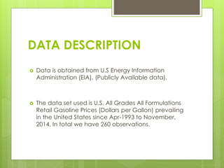
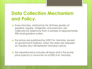
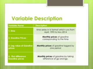
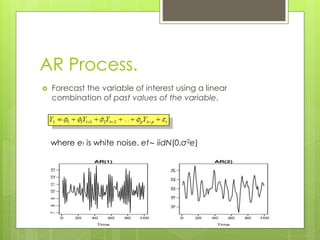
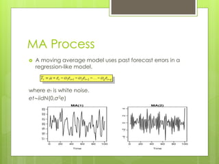
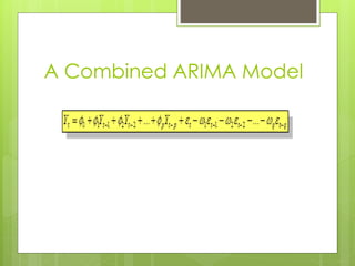
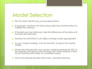
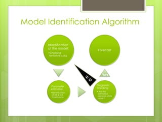
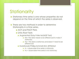
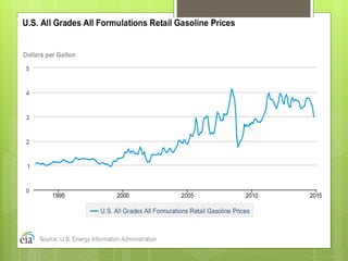
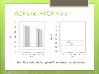
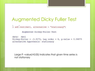
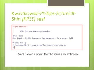
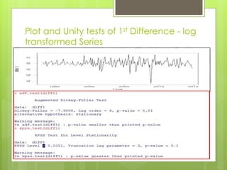
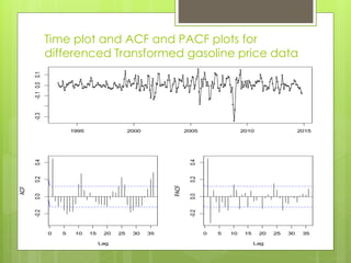
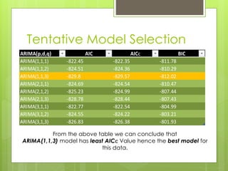
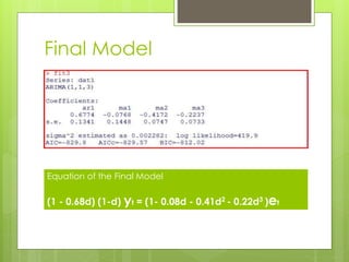
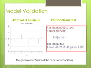
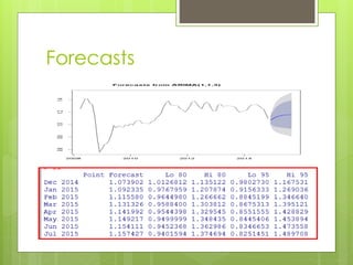
This document discusses forecasting gasoline prices in the United States using an ARIMA model. It provides background on gasoline, including its consumption and retail prices. The objective is to understand price volatility due to supply and demand constraints. Data on US gasoline prices from 1993-2014 is obtained from the EIA. After checking for stationarity and transforming the data, an ARIMA(1,1,3) model is identified as best. This model reveals gasoline prices are significantly related to past prices and unobserved factors. The validated model is used to forecast future gasoline prices.

1. Forecasting U.S
Gasoline Prices:
ARIMA Modeling
Using R
Srinivas KNS

2. Gasoline (Quick Facts)
 Gasoline or petrol is a transparent, petroleum-
derived liquid that is used primarily as a fuel in
internal combustion engines.
 A 42 gallon Crude produces19 gallons of gasoline
through Fractional Distillation.
 Some of the main components of gasoline:
isooctane, butane, 3-ethyltoluene, and the octane
enhancer MtBE.

3. Gasoline Consumption in US
 Gasoline accounts for about 66% of all the energy
used for transportation, 47% of all petroleum
consumption, and 17% of total U.S. energy
consumption.
 Consumption in 2010 was about 138 billion gallons,
an average of about 378 million gallons per day.
 63% of the crude oil for Gasoline manufacturing is
imported.

4. Retail Price of Gasoline and its
components.
Ave retail
price till
2013 is 3.43
Ave retail
price in 2013
is 3.58

5. Objective of the ANALYSIS
 To Understand Price volatility due supply and
Demand Constraints.
 The study on gasoline price will help to design better
options for pricing mechanism for markets.
 Trend estimates allow the investigation of empirical
regularities that characterize the gasoline markets.

6. DATA DESCRIPTION
 Data is obtained from U.S Energy Information
Administration (EIA). (Publicly Available data).
 The data set used is U.S. All Grades All Formulations
Retail Gasoline Prices (Dollars per Gallon) prevailing
in the United States since Apr-1993 to November,
2014. In total we have 260 observations.

7. Data Collection Mechanism
and Policy.
 Every Monday, retail prices for all three grades of
gasoline: regular, midgrade, and premium, are
collected by telephone from a sample of approximately
900 retail gasoline outlets.
 the prices are published by 5:00 P.M. Monday, except
on government holidays, when the data are released
on tuesday (but still represent Monday's price).
 the reported price includes all taxes and is the pump
price paid by a consumer as of 8:00 A.M. Monday.

8. Variable Description
Variable Name Description
1. time
time series in ts format which runs from
April, 1993 to Nov,2014
2. Gasoline Prices
Monthly prices of gasoline
corresponding to the time
3. Lag value of Gasoline
prices
Monthly prices of gasoline lagged by
one period
4. First difference
Gasoline prices
Monthly prices of gasoline by taking
difference of gp and lgp.

9. Box Jenkins Methodology
 Box Jenkins Methodology or ARIMA Model – Auto
Regressive Integrated Moving Average Model).
 A Stochastic Modelling Approach.

10. AR Process.
 Forecast the variable of interest using a linear
combination of past values of the variable.
where et is white noise. et∼ iidN(0,σ2e)

11. MA Process
 A moving average model uses past forecast errors in a
regression-like model.
where et is white noise.
et∼iidN(0,σ2e)

12. A Combined ARIMA Model

13. Model Selection
 Plot the data. Identify any unusual observations.
 If necessary, transform the data (using a Box-Cox transformation) to
stabilize the variance.
 If the data are non-stationary: take first differences of the data until
the data are stationary.
 Examine the ACF/PACF: Is an AR(p) or MA(q) model appropriate?
 Try your chosen model(s), and use the AICc to search for a better
model.
 Check the residuals from your chosen model by plotting the ACF of
the residuals, and doing a portmanteau test of the residuals. If they
do not look like white noise, try a modified model.
 Once the residuals look like white noise, calculate forecasts.

14. Model Identification Algorithm
Identification
of the model:
•Choosing
tentative p,d,q
Parameter
estimation
•Identification
of AR & MA
Coefficients
Diagnostic
checking
• Are the
estimated
residuals white
noise ?
Forecast
Yes

15. Stationarity
 Stationary time series is one whose properties do not
depend on the time at which the series is observed.
 There are two methods in order to determine
Stationarity in a time series.
 ACF and PACF Plots
 Unity Root Tests
 Augmented Dicky Fuller test(ADF Test)
 H0 = the data needs to be differenced to make it
stationary
 Ha = the data is stationary and doesn’t need to be
differenced
 Kwiatkowski-Phillips-Schmidt-Shin (KPSS)test
 H0 = observable time series is stationary
 Ha = observable time series is not stationary

16. Diagnostic Checking
 There are Two ways to check for the
residuals.
 ACF of Residuals to see that there are no
correlations in the residuals
 portmanteau test
 H0: The data are independently distributed
 Ha: The data are not independently distributed.

18. ACF and PACF Plots
Both Plots Indicate that given Time series is non stationary

19. Augmented Dicky Fuller Test
Large P –value(>0.05) Indicates that given time series is
not stationary

20. Kwiatkowski-Phillips-Schmidt-
Shin (KPSS) test
Small P value suggests that the series is not stationary

21. Observations from the Initial
Analysis.
 Given Time series is not Stationary
 Log Transformation of the series is required
in order to stabilize the variance.

22. Transformation and Tentative
Model Selection.
 Applying Log Transformation.
 Taking First Difference of the transformed
Data.
 Different models are chosen to minimize
the Aicc values.

23. Plot and Unity tests of 1st Difference - log
transformed Series

24. 1995 2000 2005 2010 2015
-0.3-0.10.00.1
0 5 10 15 20 25 30 35
-0.20.00.20.4
Lag
ACF
0 5 10 15 20 25 30 35
-0.20.00.20.4
Lag
PACF
Time plot and ACF and PACF plots for
differenced Transformed gasoline price data

25. Tentative Model Selection
ARIMA(p,d,q) AIC AICC BIC
›ARIMA(1,1,1) -822.45 -822.35 -811.78
›ARIMA(1,1,2) -824.51 -824.36 -810.29
›ARIMA(1,1,3) -829.8 -829.57 -812.02
›ARIMA(2,1,1) -824.69 -824.54 -810.47
›ARIMA(2,1,2) -825.23 -824.99 -807.44
›ARIMA(2,1,3) -828.78 -828.44 -807.43
›ARIMA(3,1,1) -822.77 -822.54 -804.99
›ARIMA(3,1,2) -824.55 -824.22 -803.21
›ARIMA(3,1,3) -826.83 -826.38 -801.93
From the above table we can conclude that
ARIMA(1,1,3) model has least AICC Value hence the best model for
this data.

26. Final Model
Equation of the Final Model
(1 - 0.68d) (1-d) yt = (1- 0.08d - 0.41d2
- 0.22d3
)et

27. Model Validation
ACF plot of Residuals Portmanteau test
The given Model Satisfy all the necessary conditions

28. Forecasts

29. Conclusion
 ARIMA(1,1,3) reveals significant coefficients for all
lags in the AR process, which basically implies that
gasoline prices in period t are significantly related
with past period gasoline price levels.
 On the other hand error term (MA process) has
also significant coefficients for all (3 in this case)
last period error values. That clearly reveals the
fact that gasoline prices are significantly related to
both the past period price levels and to
unobserved factors.
 This is the fact that has resulted in terms of higher
gasoline prices under forecasting in this analysis.

30. Discussion