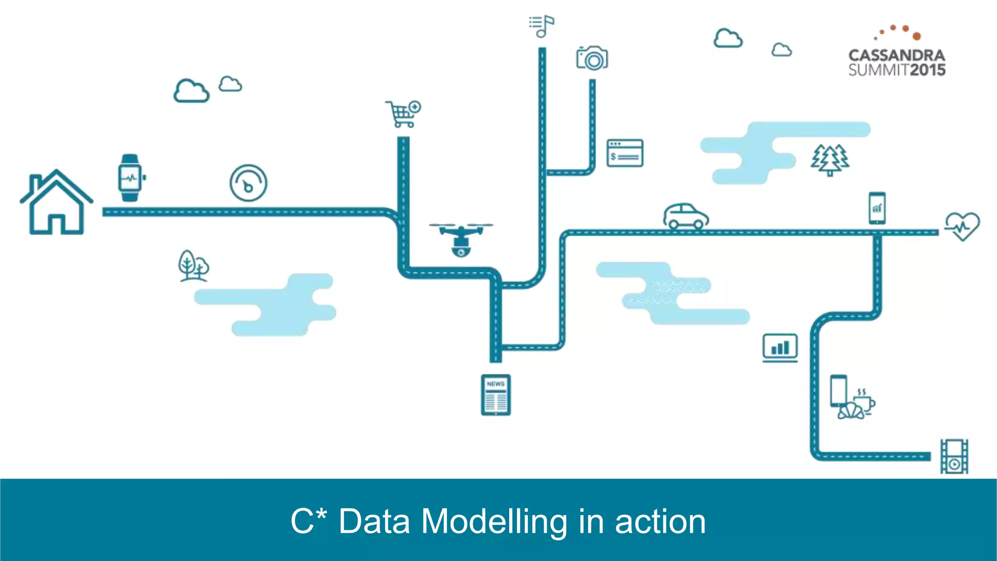
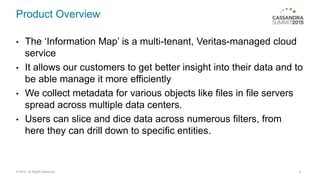
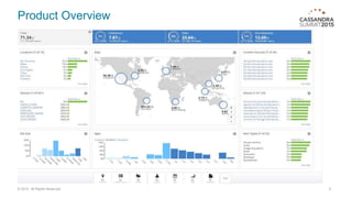
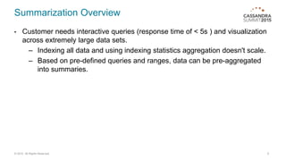
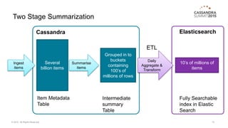
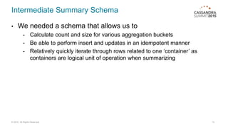
C* Data Modelling in action
1 Product Overview
2 Summarization Overview
3 Intermediate Summary Schema
2© 2015. All Rights Reserved.
Product Overview
© 2015. All Rights Reserved. 3
Product Overview
• The ‘Information Map’ is a multi-tenant, Veritas-managed cloud
service
• It allows our customers to get better insight into their data and to
be able manage it more efficiently
• We collect metadata for various objects like files in file servers
spread across multiple data centers.
• Users can slice and dice data across numerous filters, from
here they can drill down to specific entities.
4© 2015. All Rights Reserved.
Product Overview
5© 2015. All Rights Reserved.
C* Cluster
• 18 Node C* Cluster
– AWS Instance type – i2.2xlarge
– 8 vCPU
– 60 GB RAM
– 1.6 TB SSD (2 * 800)
• C* cluster stats
- 5 billion items total, average 300 million per customer, largest customer
has 1.9 billion items
- 380 GB – 410 GB per node (total ~ 7 TB across cluster)
6© 2015. All Rights Reserved.
C* Cluster
7© 2015. All Rights Reserved.
Summarization Overview
© 2015. All Rights Reserved. 8
Summarization Overview
• Customer needs interactive queries (response time of < 5s ) and visualization
across extremely large data sets.
– Indexing all data and using indexing statistics aggregation doesn't scale.
– Based on pre-defined queries and ranges, data can be pre-aggregated
into summaries.
9© 2015. All Rights Reserved.
Two Stage Summarization
ElasticsearchCassandra
10© 2015. All Rights Reserved.
Several
billion items
Ingest
items
Grouped in to
buckets
containing
100’s of
millions of rows
Item Metadata
Table
Intermediate
summary
Table
Daily
Aggregate &
Transform
10’s of millions of
items
Fully Searchable
index in Elastic
Search
Summarise
items
ETL
Summary Data - Example
11© 2015. All Rights Reserved.
Item
Id
Location Content
Source
(file server)
Container
(Share)
Size FileType Creation Date
1 Reading Server1 Share1 100 KB Word 17/09/2015
2 Reading Server1 Share1 80 KB Word 18/09/2015
3 NewYork Server2 Share2 150 KB Excel 11/01/2015
4 NewYork Server2 Share2 150 KB Excel 13/01/2015
5 NewYork Server2 Share2 600 KB Excel 13/02/2015
Location Content Source
(file server)
Container
(share)
Age Bucket
(relative today)
FileType Total
Count
Total
Size
Reading Server1 Share1 Last Month Word 2 180 KB
NewYork Server2 Share2 Last Year Excel 3 1000 KB
Container
(Share)
Weekly Bucket
(from 01-01-2015)
FileType Items with Size
Share1 37 Word 1-100KB,2-80KB
Share2 2 Excel 3-150KB,4-250KB
Share2 7 Excel 5-600KB
Item Metadata (Cassandra)
1st Stage summarization (Cassandra)
2nd Stage summarization (Elasticsearch)
© 2015. All Rights Reserved. 12
Intermediate Summary Schema
• We needed a schema that allows us to
- Calculate count and size for various aggregation buckets
- Be able to perform insert and updates in an idempotent manner
- Relatively quickly iterate through rows related to one ‘container’ as
containers are logical unit of operation when summarizing
13© 2015. All Rights Reserved.
Making it idempotent
• Pre Cassandra 2.1 Counters are not idempotent
• Used a map to of items and size stored against bucket
combinations
– Makes it idempotent and allows navigating back to item
• First schema had
– PRIMARY KEY(ContainerId,Item_Type_bucket,Size_Bucket,Owner_bucket,
cDate_Bucket, mDate_bucket,aDate_bucket)
– This uses compound primary key with ContainerId as partition key
– Allows to
• enumerate all the data for a container
• efficient slice range queries for known buckets
14© 2015. All Rights Reserved.
Problem with first attempt
• Cassandra stores data on a node by partition key.
• ContainerId as partition key leads to hotspots and excessive wide rows
15© 2015. All Rights Reserved.
Bucket_a1|Bucket_b1|bucket_c1
{itemId1,size1;
itemid2,size2;
…}
Bucket_a1|Bucket_b2|bucket_c1
{itemId3,size3;
itemid4,size4;
…}
Bucket_a1|Bucket_b1|bucket_c2
{itemId1,size1;
itemid2,size2;
…}
All other combinations
for ContainerId1
ContainerId2
Bucket_a2|Bucket_b1|bucket_c1
{itemId11,size11;
itemid12,size2;
…}
Bucket_a2|Bucket_b2|bucket_
c1
{itemId13,size13;
itemid14,size14;
…}
Bucket_a2|Bucket_b1|bucket_
c2
{itemId14,size21;
itemid15,size22;
…}
All other combinations
for ContainerId2
ContainerId1
Handling excessive wide rows
- We have pre-known combinations of item type and size buckets
- By combining them with containerId and making it composite partition key we can
reduce the physical row size.
– PRIMARY KEY ((ContainerId,Item_Type_bucket,Size_Bucket), Owner_bucket,
cDate_Bucket, mdate_bucket,aDate_bucket)
16© 2015. All Rights Reserved.
Container1/ItemType1/SizeBucket1
C1|O1|CDt1|MDt1|ADt1
{itemId1,size1;
itemid2,size2;
…}
C1|O1|CDt2|MDt2|ADt1
{itemId3,size3;
itemid4,size4;
…}
C1|O1|CDt1|MDt1|ADt1
{itemId1,size1;
itemid2,size2;
…}
All other combinations
for Container1, filetype1
& sizebucket1
C1|O1|CDt1|MDt1|ADt1
{itemId11,size11;
itemid12,size2;
…}
C1|O1|CDt2|MDt2|ADt1
{itemId13,size13;
itemid14,size14;
…}
C1|O1|CDt1|MDt1|ADt1
{itemId14,size21;
itemid15,size22;
…}
All other combinations
for container1, filetype1
& sizebucket2
Container1/ItemType2/SizeBucket2
Handling excessive wide rows – contd.
- To enumerate all the rows for a container, we make queries using all
the known combinations of ‘item type’ and ‘size bucket’ along with that
container id.
- For e.g. if there are 50 values in ‘item type’ and 10 in ‘size bucket’ then
we will make 500 queries for that container id one by one.
- For container Id1
- For each ‘item type’
- For each size ‘size bucket’
- Page through all rows from intermediate_summary table by
partition key i.e. containerId1, item_type1, size_bucket1
17© 2015. All Rights Reserved.
Handling hot spots
- Based on data profile it could still lead to hot spots
- Used ‘salt’ as part of composite partition key
- Salt derived from hashing some of the item metadata
- PRIMARY KEY ((ContainerId,Item_Type_bucket,Size_Bucket, salt),
Owner_bucket, cDate_Bucket, mdate_bucket,aDate_bucket)
- For a salt range of 1-50 we now have sub divided partition key row size by
1/50th assuming even distribution
18© 2015. All Rights Reserved.
Compaction Strategy
- Started getting lots of ReadTimeout during ETL
- nodetool cfhistogram showed many SSTables used per read
- Updates to data causing a logical row to spread into many SSTables
- Moved from default ‘SizeTiered’ to ‘Levelled’ compaction that
- Guarantees that 90% of all reads will be satisfied from a single sstable
- But uses much more I/O compared to size-tiered compaction
- We tried and found ingest rates were not impacted while ETL errors
reduced
19© 2015. All Rights Reserved.
Issue with Collection types
- Collections are read in their entirety
- Collection types are not for un-bounded scenarios and limited to 64K
- So changed the schema and now have itemId in PK
- PRIMARY KEY ((container_id, size_bucket, item_type, salt), owner_id,
cdate_bucket, mdate_bucket, adate_bucket, item_id))
- We manage client side how many items belong to same bucket
- In-memory aggregation of items using Bucket combinations
20© 2015. All Rights Reserved.
Tombstone issue
- Excess deletes are caused because item metadata change means deleting
and reinserting
- Hit more than 100K tombstones during reading
- Reduced gc_grace_seconds to 5 days in intermediate_summary
- Used a separate ‘repair’ script for intermediate_summary to be run every 3
days
- Changed schema again to do aggregation per partition key and take dates out
of PK
- PRIMARY KEY ((container_id, size_bucket, item_type, salt), owner_id, item_id)) – date
buckets just non key columns
- In-memory aggregation of items using (container_id, size_bucket, item_type, salt) combinations
21© 2015. All Rights Reserved.
Thank you

Symantec: Cassandra Data Modelling techniques in action

  • 1.
  • 2.
    1 Product Overview 2Summarization Overview 3 Intermediate Summary Schema 2© 2015. All Rights Reserved.
  • 3.
    Product Overview © 2015.All Rights Reserved. 3
  • 4.
    Product Overview • The‘Information Map’ is a multi-tenant, Veritas-managed cloud service • It allows our customers to get better insight into their data and to be able manage it more efficiently • We collect metadata for various objects like files in file servers spread across multiple data centers. • Users can slice and dice data across numerous filters, from here they can drill down to specific entities. 4© 2015. All Rights Reserved.
  • 5.
    Product Overview 5© 2015.All Rights Reserved.
  • 6.
    C* Cluster • 18Node C* Cluster – AWS Instance type – i2.2xlarge – 8 vCPU – 60 GB RAM – 1.6 TB SSD (2 * 800) • C* cluster stats - 5 billion items total, average 300 million per customer, largest customer has 1.9 billion items - 380 GB – 410 GB per node (total ~ 7 TB across cluster) 6© 2015. All Rights Reserved.
  • 7.
    C* Cluster 7© 2015.All Rights Reserved.
  • 8.
    Summarization Overview © 2015.All Rights Reserved. 8
  • 9.
    Summarization Overview • Customerneeds interactive queries (response time of < 5s ) and visualization across extremely large data sets. – Indexing all data and using indexing statistics aggregation doesn't scale. – Based on pre-defined queries and ranges, data can be pre-aggregated into summaries. 9© 2015. All Rights Reserved.
  • 10.
    Two Stage Summarization ElasticsearchCassandra 10©2015. All Rights Reserved. Several billion items Ingest items Grouped in to buckets containing 100’s of millions of rows Item Metadata Table Intermediate summary Table Daily Aggregate & Transform 10’s of millions of items Fully Searchable index in Elastic Search Summarise items ETL
  • 11.
    Summary Data -Example 11© 2015. All Rights Reserved. Item Id Location Content Source (file server) Container (Share) Size FileType Creation Date 1 Reading Server1 Share1 100 KB Word 17/09/2015 2 Reading Server1 Share1 80 KB Word 18/09/2015 3 NewYork Server2 Share2 150 KB Excel 11/01/2015 4 NewYork Server2 Share2 150 KB Excel 13/01/2015 5 NewYork Server2 Share2 600 KB Excel 13/02/2015 Location Content Source (file server) Container (share) Age Bucket (relative today) FileType Total Count Total Size Reading Server1 Share1 Last Month Word 2 180 KB NewYork Server2 Share2 Last Year Excel 3 1000 KB Container (Share) Weekly Bucket (from 01-01-2015) FileType Items with Size Share1 37 Word 1-100KB,2-80KB Share2 2 Excel 3-150KB,4-250KB Share2 7 Excel 5-600KB Item Metadata (Cassandra) 1st Stage summarization (Cassandra) 2nd Stage summarization (Elasticsearch)
  • 12.
    © 2015. AllRights Reserved. 12 Intermediate Summary Schema
  • 13.
    Intermediate Summary Schema •We needed a schema that allows us to - Calculate count and size for various aggregation buckets - Be able to perform insert and updates in an idempotent manner - Relatively quickly iterate through rows related to one ‘container’ as containers are logical unit of operation when summarizing 13© 2015. All Rights Reserved.
  • 14.
    Making it idempotent •Pre Cassandra 2.1 Counters are not idempotent • Used a map to of items and size stored against bucket combinations – Makes it idempotent and allows navigating back to item • First schema had – PRIMARY KEY(ContainerId,Item_Type_bucket,Size_Bucket,Owner_bucket, cDate_Bucket, mDate_bucket,aDate_bucket) – This uses compound primary key with ContainerId as partition key – Allows to • enumerate all the data for a container • efficient slice range queries for known buckets 14© 2015. All Rights Reserved.
  • 15.
    Problem with firstattempt • Cassandra stores data on a node by partition key. • ContainerId as partition key leads to hotspots and excessive wide rows 15© 2015. All Rights Reserved. Bucket_a1|Bucket_b1|bucket_c1 {itemId1,size1; itemid2,size2; …} Bucket_a1|Bucket_b2|bucket_c1 {itemId3,size3; itemid4,size4; …} Bucket_a1|Bucket_b1|bucket_c2 {itemId1,size1; itemid2,size2; …} All other combinations for ContainerId1 ContainerId2 Bucket_a2|Bucket_b1|bucket_c1 {itemId11,size11; itemid12,size2; …} Bucket_a2|Bucket_b2|bucket_ c1 {itemId13,size13; itemid14,size14; …} Bucket_a2|Bucket_b1|bucket_ c2 {itemId14,size21; itemid15,size22; …} All other combinations for ContainerId2 ContainerId1
  • 16.
    Handling excessive widerows - We have pre-known combinations of item type and size buckets - By combining them with containerId and making it composite partition key we can reduce the physical row size. – PRIMARY KEY ((ContainerId,Item_Type_bucket,Size_Bucket), Owner_bucket, cDate_Bucket, mdate_bucket,aDate_bucket) 16© 2015. All Rights Reserved. Container1/ItemType1/SizeBucket1 C1|O1|CDt1|MDt1|ADt1 {itemId1,size1; itemid2,size2; …} C1|O1|CDt2|MDt2|ADt1 {itemId3,size3; itemid4,size4; …} C1|O1|CDt1|MDt1|ADt1 {itemId1,size1; itemid2,size2; …} All other combinations for Container1, filetype1 & sizebucket1 C1|O1|CDt1|MDt1|ADt1 {itemId11,size11; itemid12,size2; …} C1|O1|CDt2|MDt2|ADt1 {itemId13,size13; itemid14,size14; …} C1|O1|CDt1|MDt1|ADt1 {itemId14,size21; itemid15,size22; …} All other combinations for container1, filetype1 & sizebucket2 Container1/ItemType2/SizeBucket2
  • 17.
    Handling excessive widerows – contd. - To enumerate all the rows for a container, we make queries using all the known combinations of ‘item type’ and ‘size bucket’ along with that container id. - For e.g. if there are 50 values in ‘item type’ and 10 in ‘size bucket’ then we will make 500 queries for that container id one by one. - For container Id1 - For each ‘item type’ - For each size ‘size bucket’ - Page through all rows from intermediate_summary table by partition key i.e. containerId1, item_type1, size_bucket1 17© 2015. All Rights Reserved.
  • 18.
    Handling hot spots -Based on data profile it could still lead to hot spots - Used ‘salt’ as part of composite partition key - Salt derived from hashing some of the item metadata - PRIMARY KEY ((ContainerId,Item_Type_bucket,Size_Bucket, salt), Owner_bucket, cDate_Bucket, mdate_bucket,aDate_bucket) - For a salt range of 1-50 we now have sub divided partition key row size by 1/50th assuming even distribution 18© 2015. All Rights Reserved.
  • 19.
    Compaction Strategy - Startedgetting lots of ReadTimeout during ETL - nodetool cfhistogram showed many SSTables used per read - Updates to data causing a logical row to spread into many SSTables - Moved from default ‘SizeTiered’ to ‘Levelled’ compaction that - Guarantees that 90% of all reads will be satisfied from a single sstable - But uses much more I/O compared to size-tiered compaction - We tried and found ingest rates were not impacted while ETL errors reduced 19© 2015. All Rights Reserved.
  • 20.
    Issue with Collectiontypes - Collections are read in their entirety - Collection types are not for un-bounded scenarios and limited to 64K - So changed the schema and now have itemId in PK - PRIMARY KEY ((container_id, size_bucket, item_type, salt), owner_id, cdate_bucket, mdate_bucket, adate_bucket, item_id)) - We manage client side how many items belong to same bucket - In-memory aggregation of items using Bucket combinations 20© 2015. All Rights Reserved.
  • 21.
    Tombstone issue - Excessdeletes are caused because item metadata change means deleting and reinserting - Hit more than 100K tombstones during reading - Reduced gc_grace_seconds to 5 days in intermediate_summary - Used a separate ‘repair’ script for intermediate_summary to be run every 3 days - Changed schema again to do aggregation per partition key and take dates out of PK - PRIMARY KEY ((container_id, size_bucket, item_type, salt), owner_id, item_id)) – date buckets just non key columns - In-memory aggregation of items using (container_id, size_bucket, item_type, salt) combinations 21© 2015. All Rights Reserved.
  • 22.

Editor's Notes

  • #10 Idea is to create a pre-aggregated view using known ranges and combinations and then run the search on this aggregated view of data rather than running it on entire dataset of billions of items
  • #15 With Counter column family, if you get a timeout error there is no guarantee that operation didn’t eventually completed. PK has two parts - partition key and clustering key A compound primary key includes the partition key, which determines on which node data is stored, and one or more additional columns that determine clustering. Cassandra uses the first column name in the primary key definition as the partition key The remaining column, or columns that are not partition keys in the primary key definition are the clustering columns. The data for each partition is clustered by the remaining column or columns of the primary key definition. On a physical node, when rows for a partition key are stored in order based on the clustering columns, retrieval of rows is very efficient. Essentially, the clustering columns determine the on-disk sort order within each partition.  The column to designate as the partition key largely depends on the requirements of the application and the particular query you are trying to solve.  Be mindful of the cardinality of your potential partition key.  If it is too low you will get “hot spots” (poor data distribution), and if it is too high you will negate the benefits of the “wide row” data model (too little data to make ordering worthwhile).
  • #16 Rules of C* Data modelling 1. Spread data evenly around the cluster 2. Minimize the number of partitions read Some containers can be very large and others small. So data distribution is not uniform and can easily get hotspots. A container can easily have 100’s of millions of items and storing all that for 1 partition key make excessive wide rows. A physical row size of 10 MB is ideal may be up to 20 MB but with this schema
  • #17 Talk about Physical layout in C* http://www.datastax.com/dev/blog/schema-in-cassandra-1-1 At physical level we have partition key and then row for that partition key. Row has one cell for every non key column in that row. A partition key can be composite key with multiple components of that partition key and uses compositeComparator for multiple constituents. Cell name of the column has two parts. First part is made up of all the non partition key column values and second part is made up of non key column name, http://www.datastax.com/dev/blog/thrift-to-cql3 Refer: http://www.datastax.com/wp-content/uploads/2012/10/comments_schema.png http://www.datastax.com/dev/blog/thrift-to-cql3 In thrift land we have Static column family and Dynamic column family In thrift, a static column family is one where each internal row will have more or less the same set of cell names, and that set is finite  dynamic column family (or column family with wide rows) is one where each internal row may contain completely different sets of cells.
  • #18 Talk about Physical layout in C*
  • #19 Talk about Physical layout in C*
  • #20 Lot of updates and deletes cause row to be split across multiple SSTables. One row can have its fragments split into multiple SSTables in sizeTered compaction. The nodetool cfhistograms command provides statistics about a table, including number of SSTables, read/write latency, partition (row) size, and cell count. Nodetool cfhistogram gives histogram of number of SSTables per read Talk about SizeTier Vs Levelled Cassandra’s size-tiered compaction strategy is very similar to the one described in Google’s Bigtable paper: when enough similar-sized sstables are present (four by default), Cassandra will merge them. In figure 1, each green box represents an sstable, and the arrow represents compaction. As new sstables are created, nothing happens at first. Once there are four, they are compacted together, and again when we have another four.  Levelled compaction creates sstables of a fixed, relatively small size (5MB by default in Cassandra’s implementation), that are grouped into “levels.” Within each level, sstables are guaranteed to be non-overlapping. Each level is ten times as large as the previous. Earlier we were seeing many reads up to 8-10 SSTables, with Levelled only few needed more than 2 SSTables LeveledCompactionStrategy Works well with overwrites and tombstones. Provides low read latency
  • #21 This release (1.2) of Cassandra includes collection types that provide an improved way of handling tasks, such as building multiple email address capability into tables. Observe the following limitations of collections:The maximum size of an item in a collection is 64K. Keep collections small to prevent delays during querying because Cassandra reads a collection in its entirety. The collection is not paged internally.As discussed earlier, collections are designed to store only a small amount of data. Never insert more than 64K items in a collection.If you insert more than 64K items into a collection, only 64K of them will be queryable, resulting in data loss. You can expire each element of a collection by setting an individual time-to-live (TTL) property. http://docs.datastax.com/en/cql/3.0/cql/cql_using/use_collections_c.html