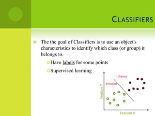
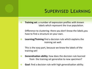
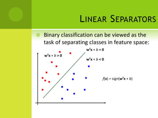
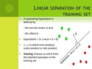
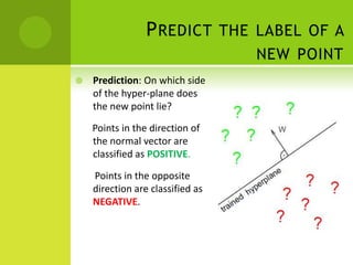
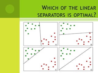
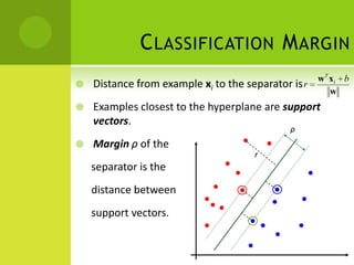
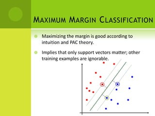
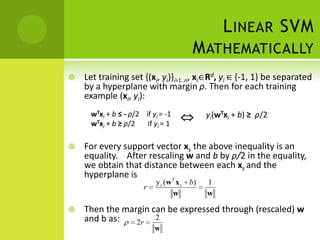
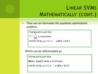
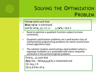
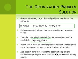
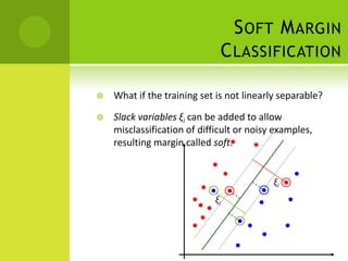
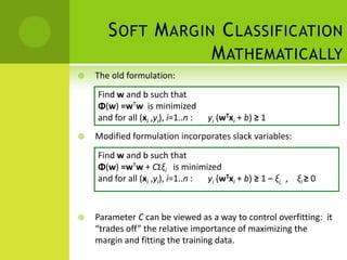
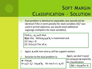
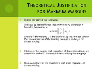
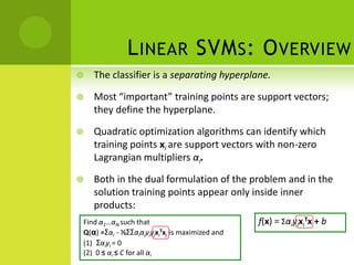
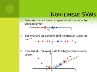
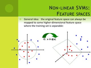
The document discusses support vector machines (SVMs) for classification. It begins by defining classifiers and the difference between classification and clustering. It then introduces SVMs, explaining that they find optimal decision boundaries that separate classes through mapping data points into higher dimensional space. The document outlines linear and non-linear SVMs, describing how non-linear SVMs can find more complex separating structures through kernels. It also discusses supervised learning with SVMs and how to solve the optimization problem to train linear SVMs, including soft-margin classification to handle non-separable data.

1. B Y :-

2. CONTENTS
 Classifiers
 Difference b/w Classification and Clustering
 What is SVM
 Supervised learning
 Linear SVM
 NON Linear SVM
 Features and Application

3. C LASSIFIERS
 The the goal of Classifiers is to use an object's
characteristics to identify which class (or group) it
belongs to.
 Have labels for some points
 Supervised learning
Genes
Proteins
Feature Y
Feature X

4. D IFFERENCE B / W C LASSIFICATION
AND C LUSTERING
 In general, in classification you have a set of
predefined classes and want to know which class
a new object belongs to.
 Clustering tries to group a set of object.
 In the context of machine learning, classification
is supervised learning and clustering
is unsupervised learning.

5. W HAT I S SVM?
 Support Vector Machines are based on the
concept of decision planes that define decision
boundaries.
 A decision plane is one that separates between a
set of objects having different class
memberships.

6.  the objects belong either to class GREEN or RED.
 The separating line defines a boundary on the right side of
which all objects are GREEN and to the left of which all
objects are RED. Any new object (white circle) falling to
the right is labeled, i.e., classified, as GREEN (or classified
as RED should it fall to the left of the separating line).
 This is a classic example of a linear classifier

7.  Most classification tasks are not as simple, as we have
seen in previous example
 More complex structures are needed in order to make an
optimal separation
 Full separation of the GREEN and RED objects would
require a curve (which is more complex than a line).

9.  In fig. we can see the original objects (left side of the
schematic) mapped, i.e., rearranged, using a set of
mathematical functions, known as kernels.
 The process of rearranging the objects is known as
mapping (transformation). Note that in this new setting,
the mapped objects (right side of the schematic) is linearly
separable and, thus, instead of constructing the complex
curve (left schematic), all we have to do is to find an
optimal line that can separate the GREEN and the RED
objects.

10.  Support Vector Machine (SVM) is primarily a classier
method that performs classification tasks by
constructing hyperplanes in a multidimensional space
that separates cases of different class labels.
 SVM supports both regression and classification tasks
and can handle multiple continuous and categorical
variables. For categorical variables a dummy variable is
created with case values as either 0 or 1. Thus, a
categorical dependent variable consisting of three
levels, say (A, B, C), is represented by a set of three
dummy variables:
 A: {1 0 0}, B: {0 1 0}, C: {0 0 1}

11. S UPPORT V ECTOR M ACHINES

12. S UPERVISED L EARNING
 Training set: a number of expression profiles with known
labels which represent the true population.
Difference to clustering: there you don't know the labels,you
have to find a structure on your own.
 Learning/Training:find a decision rule which explains the
training set well.
This is the easy part, because we know the labels of the
training set!
 Generalisation ability: how does the decision rule learned
from the training set generalize to new specimen?
 Goal: find a decision rule with high generalisation ability.

13. L INEAR S EPARATORS
 Binary classification can be viewed as the
task of separating classes in feature space:
wTx + b = 0
wTx + b > 0
wTx + b < 0
f(x) = sign(wTx + b)

14. L INEAR SEPARATION OF THE
TRAINING SET
 A separating hyperplane is
defined by
- the normal vector w and
- the offset b:
 hyperplane = {x |<w,x>+ b = 0}
 <.,.> is called inner product,
scalar product or dot product.
 Training: Choose w and b from
the labelled examples in the
training set.

15. P REDICT THE LABEL OF A
NEW POINT
 Prediction: On which side
of the hyper-plane does
the new point lie?
Points in the direction of
the normal vector are
classified as POSITIVE.
Points in the opposite
direction are classified as
NEGATIVE.

16. W HICH OF THE LINEAR
SEPARATORS IS OPTIMAL ?

17. C LASSIFICATION M ARGIN
wT xi b
 Distance from example xi to the separator is r
w
 Examples closest to the hyperplane are support
vectors.
ρ
 Margin ρ of the
r
separator is the
distance between
support vectors.

18. M AXIMUM M ARGIN C LASSIFICATION
 Maximizing the margin is good according to
intuition and PAC theory.
 Implies that only support vectors matter; other
training examples are ignorable.

19. L INEAR SVM
M ATHEMATICALLY
 Let training set {(xi, yi)}i=1..n, xi Rd, yi {-1, 1} be separated
by a hyperplane with margin ρ. Then for each training
example (xi, yi):
wTxi + b ≤ - ρ/2 if yi = -1 yi(wTxi + b) ≥ ρ/2
wTxi + b ≥ ρ/2 if yi = 1
 For every support vector xs the above inequality is an
equality. After rescaling w and b by ρ/2 in the equality,
we obtain that distance between each xs and the
hyperplane is T
y s ( w x s b) 1
r
w w
 Then the margin can be expressed through (rescaled) w
and b as: 2r
2
w

20. L INEAR SVM S
M ATHEMATICALLY ( CONT.)
 Then we can formulate the quadratic optimization
problem:
Find w and b such that
2
is maximized
w
and for all (xi, yi), i=1..n : yi(wTxi + b) ≥ 1
Which can be reformulated as:
Find w and b such that
Φ(w) = ||w||2=wTw is minimized
and for all (xi, yi), i=1..n : yi (wTxi + b) ≥ 1

21. S OLVING THE O PTIMIZATION
P ROBLEM
Find w and b such that
Φ(w) =wTw is minimized
and for all (xi, yi), i=1..n : yi (wTxi + b) ≥ 1
 Need to optimize a quadratic function subject to linear
constraints.
 Quadratic optimization problems are a well-known class of
mathematical programming problems for which several (non-
trivial) algorithms exist.
 The solution involves constructing a dual problem where a
Lagrange multiplier αi is associated with every inequality
constraint in the primal (original) problem:
Find α1…αn such that
Q(α) =Σαi - ½ΣΣαiαjyiyjxiTxj is maximized and
(1) Σαiyi = 0
(2) αi ≥ 0 for all αi

22. T HE O PTIMIZATION P ROBLEM
S OLUTION
 Given a solution α1…αn to the dual problem, solution to the
primal is:
w =Σαiyixi b = yk - Σαiyixi Txk for any αk > 0
 Each non-zero αi indicates that corresponding xi is a support
vector.
 Then the classifying function is (note that we don’t need w
explicitly): f(x) = ΣαiyixiTx + b
 Notice that it relies on an inner product between the test point
x and the support vectors xi – we will return to this later.
 Also keep in mind that solving the optimization problem
involved computing the inner products xiTxj between all training
points.

23. S OFT M ARGIN
C LASSIFICATION
 What if the training set is not linearly separable?
 Slack variables ξi can be added to allow
misclassification of difficult or noisy examples,
resulting margin called soft.
ξi
ξi

24. S OFT M ARGIN C LASSIFICATION
M ATHEMATICALLY
 The old formulation:
Find w and b such that
Φ(w) =wTw is minimized
and for all (xi ,yi), i=1..n : yi (wTxi + b) ≥ 1
 Modified formulation incorporates slack variables:
Find w and b such that
Φ(w) =wTw + CΣξi is minimized
and for all (xi ,yi), i=1..n : yi (wTxi + b) ≥ 1 – ξi, , ξi ≥ 0
 Parameter C can be viewed as a way to control overfitting: it
“trades off” the relative importance of maximizing the
margin and fitting the training data.

25. S OFT M ARGIN
C LASSIFICATION – S OLUTION
 Dual problem is identical to separable case (would not be
identical if the 2-norm penalty for slack variables CΣξi2 was
used in primal objective, we would need additional
Lagrange multipliers for slack variables):
Find α1…αN such that
Q(α) =Σαi - ½ΣΣαiαjyiyjxiTxj is maximized and
(1) Σαiyi = 0
(2) 0 ≤ αi ≤ C for all αi
 Again, xi with non-zero αi will be support vectors.
 Solution to the dual problem is: Again, we don’t need
to compute w explicitly
w =Σαiyixi
for classification:
b= yk(1- ξk) - ΣαiyixiTxk for any k s.t. αk>0
f(x) = ΣαiyixiTx + b

26. T HEORETICAL J USTIFICATION
FOR M AXIMUM M ARGINS
 Vapnik has proved the following:
The class of optimal linear separators has VC dimension h
bounded from above as 2
D
h min 2
, m0 1
where ρ is the margin, D is the diameter of the smallest sphere
that can enclose all of the training examples, and m0 is the
dimensionality.
 Intuitively, this implies that regardless of dimensionality m0 we
can minimize the VC dimension by maximizing the margin ρ.
 Thus, complexity of the classifier is kept small regardless of
dimensionality.

27. L INEAR SVM S : O VERVIEW
 The classifier is a separating hyperplane.
 Most “important” training points are support vectors;
they define the hyperplane.
 Quadratic optimization algorithms can identify which
training points xi are support vectors with non-zero
Lagrangian multipliers αi.
 Both in the dual formulation of the problem and in the
solution training points appear only inside inner
products:
Find α1…αN such that f(x) = ΣαiyixiTx + b
Q(α) =Σαi - ½ΣΣαiαjyiyjxiTxj is maximized and
(1) Σαiyi = 0
(2) 0 ≤ αi ≤ C for all αi

28. N ON - LINEAR SVM S
 Datasets that are linearly separable with some noise
work out great:
0 x
 But what are we going to do if the dataset is just too
hard?
0 x
 How about… mapping data to a higher-dimensional
space: x2
0 x

29. N ON - LINEAR SVM S :
F EATURE SPACES
 General idea: the original feature space can always be
mapped to some higher-dimensional feature space
where the training set is separable:
Φ: x → φ(x)

30. P ROPERTIES OF SVM
 Flexibility in choosing a similarity function
 Sparseness of solution when dealing with
large data sets
- only support vectors are used to specify the
separating hyperplane
 Ability to handle large feature spaces
- complexity does not depend on the
dimensionality of the feature space
 Guaranteed to converge to a single global
solution

31. SVM A PPLICATIONS
 SVM has been used successfully in many real-world
problems
- text (and hypertext) categorization
- image classification
- bioinformatics (Protein classification,
Cancer classification)
- hand-written character recognition

32. T HANK Y OU