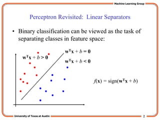
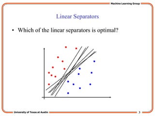
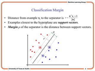
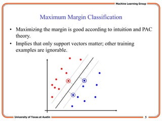
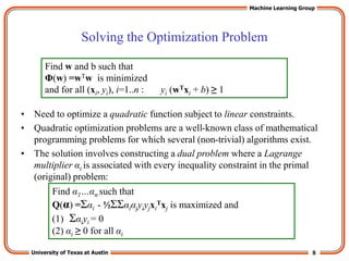
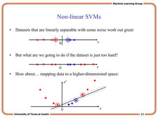
This document discusses support vector machines (SVMs) for classification tasks. It describes how SVMs find the optimal separating hyperplane with the maximum margin between classes in the training data. This is formulated as a quadratic optimization problem that can be solved using algorithms that construct a dual problem. Non-linear SVMs are also discussed, using the "kernel trick" to implicitly map data into higher-dimensional feature spaces. Common kernel functions and the theoretical justification for maximum margin classifiers are provided.

1. University of Texas at Austin
Machine Learning Group
Machine Learning Group
Department of Computer Sciences
University of Texas at Austin
Support Vector Machines

2. 2
University of Texas at Austin
Machine Learning Group
Perceptron Revisited: Linear Separators
• Binary classification can be viewed as the task of
separating classes in feature space:
wTx + b = 0
wTx + b < 0
wTx + b > 0
f(x) = sign(wTx + b)

3. 3
University of Texas at Austin
Machine Learning Group
Linear Separators
• Which of the linear separators is optimal?

4. 4
University of Texas at Austin
Machine Learning Group
Classification Margin
• Distance from example xi to the separator is
• Examples closest to the hyperplane are support vectors.
• Margin ρ of the separator is the distance between support vectors.
w
x
w b
r i
T


r
ρ

5. 5
University of Texas at Austin
Machine Learning Group
Maximum Margin Classification
• Maximizing the margin is good according to intuition and PAC
theory.
• Implies that only support vectors matter; other training
examples are ignorable.

6. 6
University of Texas at Austin
Machine Learning Group
Linear SVM Mathematically
• Let training set {(xi, yi)}i=1..n, xiRd, yi  {-1, 1} be separated by a
hyperplane with margin ρ. Then for each training example (xi, yi):
• For every support vector xs the above inequality is an equality.
After rescaling w and b by ρ/2 in the equality, we obtain that
distance between each xs and the hyperplane is
• Then the margin can be expressed through (rescaled) w and b as:
wTxi + b ≤ - ρ/2 if yi = -1
wTxi + b ≥ ρ/2 if yi = 1
w
2
2 
 r

w
w
x
w 1
)
(
y



b
r s
T
s
yi(wTxi + b) ≥ ρ/2


7. 7
University of Texas at Austin
Machine Learning Group
Linear SVMs Mathematically (cont.)
• Then we can formulate the quadratic optimization problem:
Which can be reformulated as:
Find w and b such that
is maximized
and for all (xi, yi), i=1..n : yi(wTxi + b) ≥ 1
w
2


Find w and b such that
Φ(w) = ||w||2=wTw is minimized
and for all (xi, yi), i=1..n : yi (wTxi + b) ≥ 1

8. 8
University of Texas at Austin
Machine Learning Group
Solving the Optimization Problem
• Need to optimize a quadratic function subject to linear constraints.
• Quadratic optimization problems are a well-known class of mathematical
programming problems for which several (non-trivial) algorithms exist.
• The solution involves constructing a dual problem where a Lagrange
multiplier αi is associated with every inequality constraint in the primal
(original) problem:
Find w and b such that
Φ(w) =wTw is minimized
and for all (xi, yi), i=1..n : yi (wTxi + b) ≥ 1
Find α1…αn such that
Q(α) =Σαi - ½ΣΣαiαjyiyjxi
Txj is maximized and
(1) Σαiyi = 0
(2) αi ≥ 0 for all αi

9. 9
University of Texas at Austin
Machine Learning Group
The Optimization Problem Solution
• Given a solution α1…αn to the dual problem, solution to the primal is:
• Each non-zero αi indicates that corresponding xi is a support vector.
• Then the classifying function is (note that we don’t need w explicitly):
• Notice that it relies on an inner product between the test point x and the
support vectors xi – we will return to this later.
• Also keep in mind that solving the optimization problem involved
computing the inner products xi
Txj between all training points.
w =Σαiyixi b = yk - Σαiyixi
Txk for any αk > 0
f(x) = Σαiyixi
Tx + b

10. 10
University of Texas at Austin
Machine Learning Group
Soft Margin Classification
• What if the training set is not linearly separable?
• Slack variables ξi can be added to allow misclassification of difficult or
noisy examples, resulting margin called soft.
ξi
ξi

11. 11
University of Texas at Austin
Machine Learning Group
Soft Margin Classification Mathematically
• The old formulation:
• Modified formulation incorporates slack variables:
• Parameter C can be viewed as a way to control overfitting: it “trades off”
the relative importance of maximizing the margin and fitting the training
data.
Find w and b such that
Φ(w) =wTw is minimized
and for all (xi ,yi), i=1..n : yi (wTxi + b) ≥ 1
Find w and b such that
Φ(w) =wTw + CΣξi is minimized
and for all (xi ,yi), i=1..n : yi (wTxi + b) ≥ 1 – ξi, , ξi ≥ 0

12. 12
University of Texas at Austin
Machine Learning Group
Soft Margin Classification – Solution
• Dual problem is identical to separable case (would not be identical if the 2-
norm penalty for slack variables CΣξi
2 was used in primal objective, we
would need additional Lagrange multipliers for slack variables):
• Again, xi with non-zero αi will be support vectors.
• Solution to the dual problem is:
Find α1…αN such that
Q(α) =Σαi - ½ΣΣαiαjyiyjxi
Txj is maximized and
(1) Σαiyi = 0
(2) 0 ≤ αi ≤ C for all αi
w =Σαiyixi
b= yk(1- ξk) - Σαiyixi
Txk for any k s.t. αk>0
f(x) = Σαiyixi
Tx + b
Again, we don’t need to
compute w explicitly for
classification:

13. 13
University of Texas at Austin
Machine Learning Group
Theoretical Justification for Maximum Margins
• Vapnik has proved the following:
The class of optimal linear separators has VC dimension h bounded from
above as
where ρ is the margin, D is the diameter of the smallest sphere that can
enclose all of the training examples, and m0 is the dimensionality.
• Intuitively, this implies that regardless of dimensionality m0 we can
minimize the VC dimension by maximizing the margin ρ.
• Thus, complexity of the classifier is kept small regardless of
dimensionality.
1
,
min 0
2
2













 m
D
h


14. 14
University of Texas at Austin
Machine Learning Group
Linear SVMs: Overview
• The classifier is a separating hyperplane.
• Most “important” training points are support vectors; they define the
hyperplane.
• Quadratic optimization algorithms can identify which training points xi are
support vectors with non-zero Lagrangian multipliers αi.
• Both in the dual formulation of the problem and in the solution training
points appear only inside inner products:
Find α1…αN such that
Q(α) =Σαi - ½ΣΣαiαjyiyjxi
Txj is maximized and
(1) Σαiyi = 0
(2) 0 ≤ αi ≤ C for all αi
f(x) = Σαiyixi
Tx + b

15. 15
University of Texas at Austin
Machine Learning Group
Non-linear SVMs
• Datasets that are linearly separable with some noise work out great:
• But what are we going to do if the dataset is just too hard?
• How about… mapping data to a higher-dimensional space:
0
0
0
x2
x
x
x

16. 16
University of Texas at Austin
Machine Learning Group
Non-linear SVMs: Feature spaces
• General idea: the original feature space can always be mapped to some
higher-dimensional feature space where the training set is separable:
Φ: x → φ(x)

17. 17
University of Texas at Austin
Machine Learning Group
The “Kernel Trick”
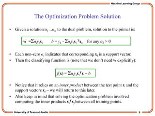
• The linear classifier relies on inner product between vectors K(xi,xj)=xi
Txj
• If every datapoint is mapped into high-dimensional space via some
transformation Φ: x → φ(x), the inner product becomes:
K(xi,xj)= φ(xi) Tφ(xj)
• A kernel function is a function that is eqiuvalent to an inner product in
some feature space.
• Example:
2-dimensional vectors x=[x1 x2]; let K(xi,xj)=(1 + xi
Txj)2
,
Need to show that K(xi,xj)= φ(xi) Tφ(xj):
K(xi,xj)=(1 + xi
Txj)2
,= 1+ xi1
2xj1
2 + 2 xi1xj1 xi2xj2+ xi2
2xj2
2 + 2xi1xj1 + 2xi2xj2=
= [1 xi1
2 √2 xi1xi2 xi2
2 √2xi1 √2xi2]T [1 xj1
2 √2 xj1xj2 xj2
2 √2xj1 √2xj2] =
= φ(xi) Tφ(xj), where φ(x) = [1 x1
2 √2 x1x2 x2
2 √2x1 √2x2]
• Thus, a kernel function implicitly maps data to a high-dimensional space
(without the need to compute each φ(x) explicitly).

18. 18
University of Texas at Austin
Machine Learning Group
What Functions are Kernels?
• For some functions K(xi,xj) checking that K(xi,xj)= φ(xi)Tφ(xj) can be
cumbersome.
• Mercer’s theorem:
Every semi-positive definite symmetric function is a kernel
• Semi-positive definite symmetric functions correspond to a semi-positive
definite symmetric Gram matrix:
K(x1,x1) K(x1,x2) K(x1,x3) … K(x1,xn)
K(x2,x1) K(x2,x2) K(x2,x3) K(x2,xn)
… … … … …
K(xn,x1) K(xn,x2) K(xn,x3) … K(xn,xn)
K=

19. 19
University of Texas at Austin
Machine Learning Group
Examples of Kernel Functions
• Linear: K(xi,xj)= xi
Txj
– Mapping Φ: x → φ(x), where φ(x) is x itself
• Polynomial of power p: K(xi,xj)= (1+ xi
Txj)p
– Mapping Φ: x → φ(x), where φ(x) has dimensions
• Gaussian (radial-basis function): K(xi,xj) =
– Mapping Φ: x → φ(x), where φ(x) is infinite-dimensional: every point is
mapped to a function (a Gaussian); combination of functions for support
vectors is the separator.
• Higher-dimensional space still has intrinsic dimensionality d (the mapping
is not onto), but linear separators in it correspond to non-linear separators
in original space.
2
2
2
j
i
e
x
x 








 
p
p
d

20. 20
University of Texas at Austin
Machine Learning Group
Non-linear SVMs Mathematically
• Dual problem formulation:
• The solution is:
• Optimization techniques for finding αi’s remain the same!
Find α1…αn such that
Q(α) =Σαi - ½ΣΣαiαjyiyjK(xi, xj) is maximized and
(1) Σαiyi = 0
(2) αi ≥ 0 for all αi
f(x) = ΣαiyiK(xi, xj)+ b

21. 21
University of Texas at Austin
Machine Learning Group
SVM applications
• SVMs were originally proposed by Boser, Guyon and Vapnik in 1992 and
gained increasing popularity in late 1990s.
• SVMs are currently among the best performers for a number of classification
tasks ranging from text to genomic data.
• SVMs can be applied to complex data types beyond feature vectors (e.g. graphs,
sequences, relational data) by designing kernel functions for such data.
• SVM techniques have been extended to a number of tasks such as regression
[Vapnik et al. ’97], principal component analysis [Schölkopf et al. ’99], etc.
• Most popular optimization algorithms for SVMs use decomposition to hill-
climb over a subset of αi’s at a time, e.g. SMO [Platt ’99] and [Joachims ’99]
• Tuning SVMs remains a black art: selecting a specific kernel and parameters is
usually done in a try-and-see manner.