A Simple Review on SVM

A Simple Review on SVM
Honglin Yu
Australian National University, NICTA
September 2, 2013

Outline
1 The Tutorial Routine
Overview
Linear SVC in Separable Case: Largest Margin Classiﬁer
Soft Margin
Solving SVM
Kernel Trick and Non-linear SVM
2 Some Topics
Why the Name: Support Vectors?
Why SVC Works Well: A Simple Example
Relation with Logistic Regression etc.
3 Packages

The Tutorial Routine Some Topics Packages
Overview
SVM (Support Vector Machines) are supervised learning
methods
It includes both methods for classiﬁcation and regression
In this talk, we focus on binary classiﬁcations.

Symbols
training data: (x1, y1), ..., (xm, ym) ∈ X × {±1}
patterns: xi , i = 1, 2, ..., m
pattern space: X
targets: yi , i = 1, 2, ..., m
features: xi = Φ(xi )
feature space: H
feature mapping: Φ : X → H

Separable Case: Largest Margin Classiﬁer
Figure: Simplest Case
“Separable” means: ∃ line
w · x + b = 0 correctly separates all
the training data.
“Margin”: d+ + d−
(d± = min
yi =±1
dist(xi , w · x + b = 0))
In this case, the SVC just looks for
a line maximizing the margins.

Separable Case: Largest Margin Classiﬁer
Another form of expressing separable: yi (w · xi + b) > 0
Because the training data is ﬁnite, ∃ , yi (w · xi + b) ≥
This is equivalent to yi (w
· xi + b
) ≥ 1
w · xi + b = 0 and w
· xi + b
= 0 are same line.
We can directly write the constraints as yi (w · xi + b) ≥ 1
This removes the scaling redundancy in w, b

We also want the separating plane to place in the middle
(which means d+ = d−).
So the optimization problem can be formulated as
arg max
w,b
(2 min
x
|w · xi + b|
|w|
)
s.t. yi (w · xi + b) ≥ 1, i = 1, 2, ..., N
(1)
This is equivalent to:
arg min
w,b
|w|2
s.t. yi (w · xi + b) ≥ 1, i = 1, 2, ..., N
(2)
But, until now, it can only be conﬁrmed that Eq.2 is only the
necessary condition of ﬁnding the plane we want (correct and
in the middle)

Largest Margin Classiﬁer
It can be proved that, when the data is separable, for the following
problem
min
w,b
1
2
||w||2
s.t. yi · (w · xi + b) ≥ 1, i = 1, ..., m.
(3)
we have,
1 When the ||w|| is minimized, the equality holds for some x.
2 The equality holds at least for some xi , xj where yi yj < 0.
3 Based on 1) and 2) we can calculate that the margin is 2
||w|| ,
so the margin is maximized.

Proof of Previous Slide (Warning: My Proof)
1 If ∃c > 1 that ∀xi , yi · (w · xi + b) ≥ c, then w
c and b
c also
satisfy the constraints and the length is smaller.
2 If not, assume that ∃c > 1,
yi · (w · xi + b) ≥ 1, where yi = 1
yi · (w · xi + b) ≥ c, where yi = −1
(4)
Add c−1
2 to each side where yi = 1, minus c−1
2 to each side
where yi = −1, we can get:
yi · (w · xi + b +
c − 1
2
) ≥
c + 1
2
(5)
Because c+1
2 > 1, similar to 1), the |w| here is not the
smallest
3 Pick x1, x2 where the equality holds and y1y2 < 0, the margin
is just the distance between x1 and the line y2 · (w · x + b) = 1
which can be easily calculated as 2
||w|| .

Non Separable Case
Figure: Non separable case: miss classiﬁed points exist

Non Separable Case
Constraints yi (w · xi + b) ≥ 1, i = 1, 2, ..., m can not be
satisﬁed
Solution: add slack variables ξi , reformulate form problem as,
min
w,b,ξ
1
2
||w||2
+ C
m
i=1
ξi
s.t. yi ((w · xi) + b) ≥ 1 − ξi , i = 1, 2, ..., m
ξi ≥ 0
(6)
Show the trade oﬀ (C) between margins ( 1
|w| ) and penalty (ξi ).

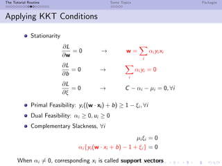
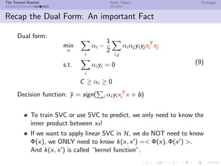
Solving SVM: Lagrangian Dual
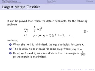
Constraint optimization → Lagrangian Dual
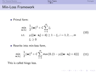
Primal form:
min
w,b,ξ
1
2
||w||2
+ C
m
i=1
ξi
s.t. yi ((w · xi) + b) ≥ 1 − ξi , i = 1, 2, ..., m
ξi ≥ 0
(7)
The Primal Lagrangian:
L(w, b, ξ, α, µ) =
1
2
||w||2
+C
i
ξi −
i
αi {yi (w·x+b−1−ξi )}−
i
µi ξi
Because [7] is convex, Karush-Kuhn-Tucker conditions hold.

Applying KKT Conditions
Stationarity
∂L
∂w
= 0 → w =
i
αi yi xi
∂L
∂b
= 0 →
i
αi yi = 0
∂L
∂ξ
= 0 → C − αi − µi = 0, ∀i
Primal Feasibility: yi ((w · xi) + b) ≥ 1 − ξi , ∀i
Dual Feasibility: αi ≥ 0, ui ≥ 0
Complementary Slackness, ∀i
µi ξi = 0
αi {yi (w · xi + b) − 1 + ξi } = 0
When αi = 0, corresponding xi is called support vectors

Dual Form
Using the equations derived from KKT conditions, remove
w, b, ξi , µi in the primal form to get the dual form:
min
α
i
αi −
1
2
i,j
αi αj yi yj xT
i xj
s.t.
i
αi yi = 0
C ≥ αi ≥ 0
(8)
And the decision function is:¯y = sign( i αi yi xT
i x + b)
(b = yk − w · xk, ∀k, C > αk > 0)

We Need Nonlinear Classiﬁer
-1
-0.5
0
0.5
1
-1 -0.5 0 0.5 1
Figure: Case that linear classiﬁer can not handle
Finding appropriate form of curves is hard, but we can transform
the data!

Mapping Training Data to Feature Space
Φ(x) = (x, x2)T
Figure: Feature Mapping Helps Classification
To solve nonlinear classification problem, we can define some
mapping Φ : X → H and do linear classification on feature space
H

Recap the Dual Form: An important Fact
Dual form:
min
α
i
αi −
1
2
i,j
αi αj yi yj xT
i xj
s.t.
i
αi yi = 0
C ≥ αi ≥ 0
(9)
Decision function: ¯y = sign( i αi yi xT
i x + b)
To train SVC or use SVC to predict, we only need to know the
inner product between xs!
If we want to apply linear SVC in H, we do NOT need to know
Φ(x), we ONLY need to know k(x, x ) =< Φ(x), Φ(x ) >.
And k(x, x ) is called “kernel function”.

Kernel Functions
The input of kernel function k : X × X → R is two patterns
x, x in X, the output is the canonical inner product between
Φ(x), Φ(x ) in H
By using k(·, ·), we can implicitly transform the data by some
Φ(·) (which is often with inﬁnite dimension) E.g. for
k(x, x ) = (xx + 1)2, Φ(x) = (x2,
√
2x, 1)T
But not for all functions X × X → R, we can ﬁnd
corresponding Φ(x). Kernel functions should satisfy Mercer’s
conditions

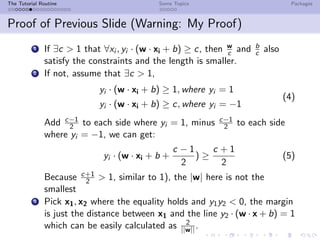
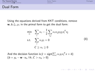
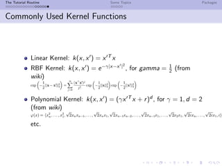
Conditions of Kernel Functions
Necessity: Kernel Matrix K = [k(xi , xj )]m×m must be positive
semidefinite:
tT
Kt =
i,j
ti tj k(xi , xj ) =
i,j
ti tj < Φ(xi ), Φ(xj ) >
=<
i
ti Φ(xi ),
j
tj Φ(xj ) >= |
i
ti Φ(xi )|2
≥ 0
Sufficiency in Continuous Form: Mercer’s Condition:
For any symmetric function k : X × X → R which is square
integrable in X × X, if it satisfies
X×X
k(x, x )f (x)f (x )dxdx ≥ 0 for all f ∈ L2(X)
there exist functions φi : X → R and numbers λi ≥ 0 that,
k(x, x ) =
i
λi φi (x)φi (x ) for all x, x in X

Commonly Used Kernel Functions
Linear Kernel: k(x, x ) = x T x
RBF Kernel: k(x, x ) = e−γ|x−x |2
, for gamma = 1
2 (from
wiki)
Polynomial Kernel: k(x, x ) = (γx T x + r)d , for γ = 1, d = 2
(from wiki)
etc.

Mechanical Analogy
Remember from KKT conditions,
∂L
∂w
= 0 → w =
i
αi yi xi
∂L
∂w
= 0 →
i
αi yi = 0
imagine every support vector xi exerts a force Fi = αi yi
w
|w| on
the “separating plane + margin”, we have,
Forces =
i
αi yi
w
|w|
=
w
|w|
i
αi yi = 0
Torques =
i
xi × (αi yi
w
|w|
) = (
i
αi yi xi ) ×
w
|w|
= w ×
w
|w|
= 0
This is why {xi } are called “support vectors”

Why SVC Works Well
Let’s first consider using linear regression to do classification, the
decision function is ¯y = sign(w · x + b)
Figure: Feature Mapping Helps Classification
In SVM, we only considers about the boundaries

Min-Loss Framework
Primal form:
min
w,b,ξ
1
2
||w||2
+ C
m
i=1
ξi
s.t. yi ((w · xi) + b) ≥ 1 − ξi , i = 1, 2, ..., m
ξi ≥ 0
(10)
Rewrite into min-loss form,
min
w,b,ξ
1
2
||w||2
+ C
m
i=1
max{0, (1 − yi ((w · xi) + b))} (11)
This is called hinge loss.

See C-SVM and LMC from a Uniﬁed Direction
Rewriting LMC classiﬁer,
min
w
1
2
||w||2
+
m
i=0
∞ · (sign(1 − y(w · xi + b)) + 1) (12)
Regularised Logistic Regression
(y ∈ {0, 1}, not {−1, 1}, pi = 1
1+e−w·xi
)
min
w
1
2
||w||2
+
m
i=0
−(yi log(pi ) + (1 − yi )log(1 − pi )) (13)

Relation with Logistic Regression etc.
Figure: black:0-1 loss; red: logistic loss (−log( 1
1+e−yi w·x )); blue: hinge
loss; green: quadratic loss.
“0-1 loss” and “hinge loss” are not aﬀected by correctly
classiﬁed outliers.
BTW, logistic regression can also be “kernelised”.

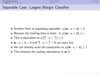
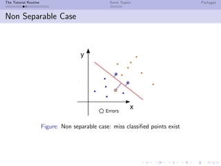
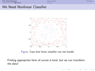
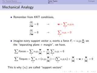
Commonly Used Packages
libsvm(liblinear), svmlight and sklearn (python wrap-up of
libsvm)
Code example in sklearn
import numpy as np
X = np . a r r a y ([[ −1 , −1] , [ −2 , −1] , [ 1 , 1 ] , [ 2 , 1 ] ] )
y = np . a r r a y ( [ 1 , 1 , 2 , 2 ] )
from s k l e a r n . svm import SVC
c l f = SVC()
c l f . f i t (X, y )
c l f . p r e d i c t ([[ −0.8 , −1]])

Things Not Covered
Algorithms (SMO, SGD)
Generalisation bound and VC dimension
ν-SVM, one-class SVM etc.
SVR
etc.

A Simple Review on SVM

More Related Content

What's hot

Similar to A Simple Review on SVM

Recently uploaded

A Simple Review on SVM