Download to read offline
![• The linear classifier relies on inner product between vectors K(xi,xj) = xi
Txj
• If every datapoint is mapped into high-dimensional space via some transformation Φ: x → φ(x), the inner
product becomes: K(xi,xj)= φ(xi) Tφ(xj)
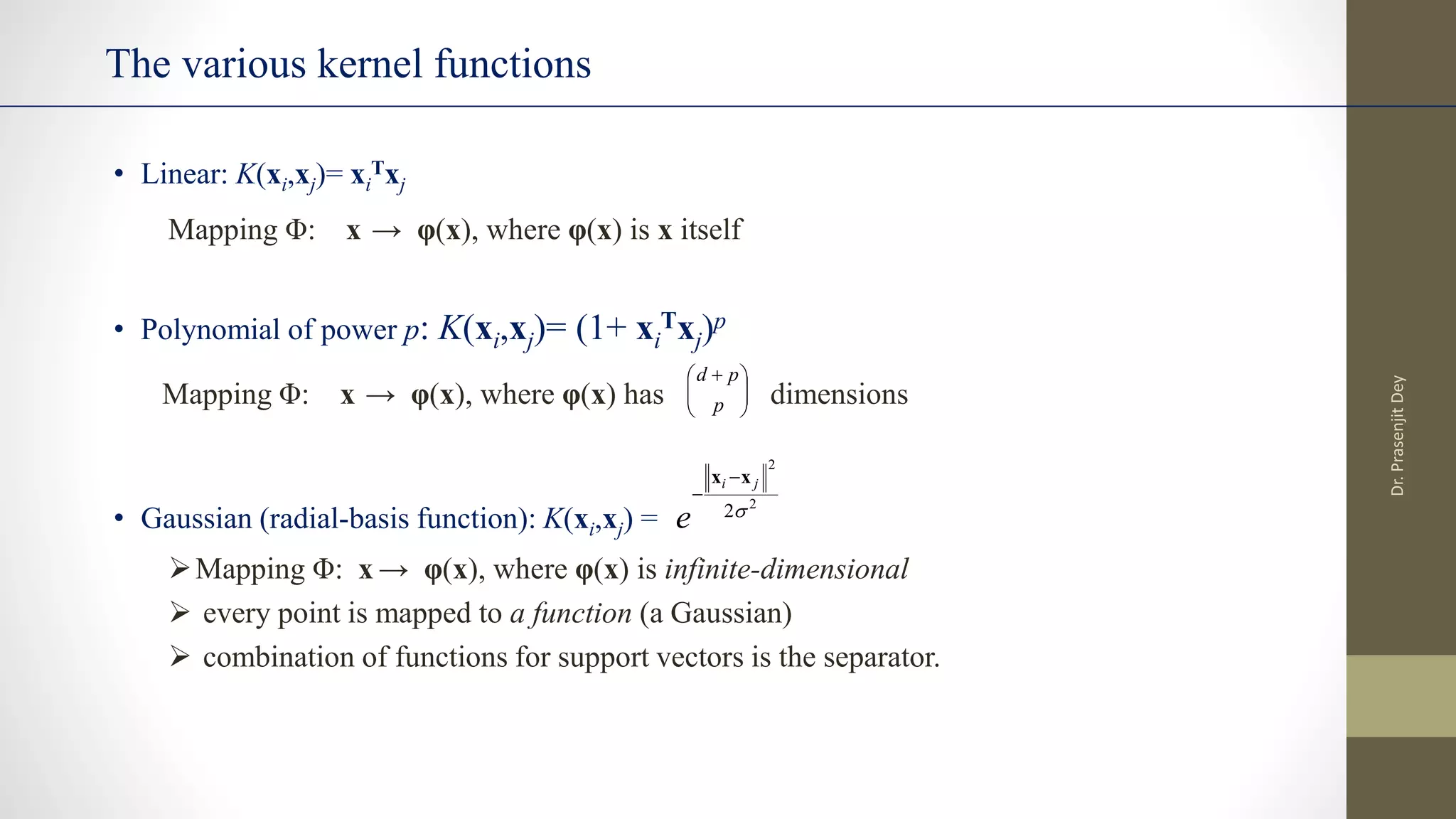
• A kernel function is a function that is equivalent to an inner product in some feature space.
• Example: 2-dimensional vectors x=[x1 x2]; let K(xi,xj) = (1 + xi
Txj)2
,
Need to show that K(xi,xj) = φ(xi) Tφ(xj):
K(xi,xj)=(1 + xi
Txj)2
,= 1+ xi1
2xj1
2 + 2 xi1xj1 xi2xj2+ xi2
2xj2
2 + 2xi1xj1 + 2xi2xj2=
= [1 xi1
2 √2 xi1xi2 xi2
2 √2xi1 √2xi2]T [1 xj1
2 √2 xj1xj2 xj2
2 √2xj1 √2xj2] =
= φ(xi) Tφ(xj), where φ(x) = [1 x1
2 √2 x1x2 x2
2 √2x1 √2x2]
• Thus, a kernel function implicitly maps data to a high-dimensional space (without the need to compute
each φ(x) explicitly).
The Kernel Functions
Dr.
Prasenjit
Dey](https://image.slidesharecdn.com/supportvectormachine-210704195413/75/Support-vector-machine-11-2048.jpg)
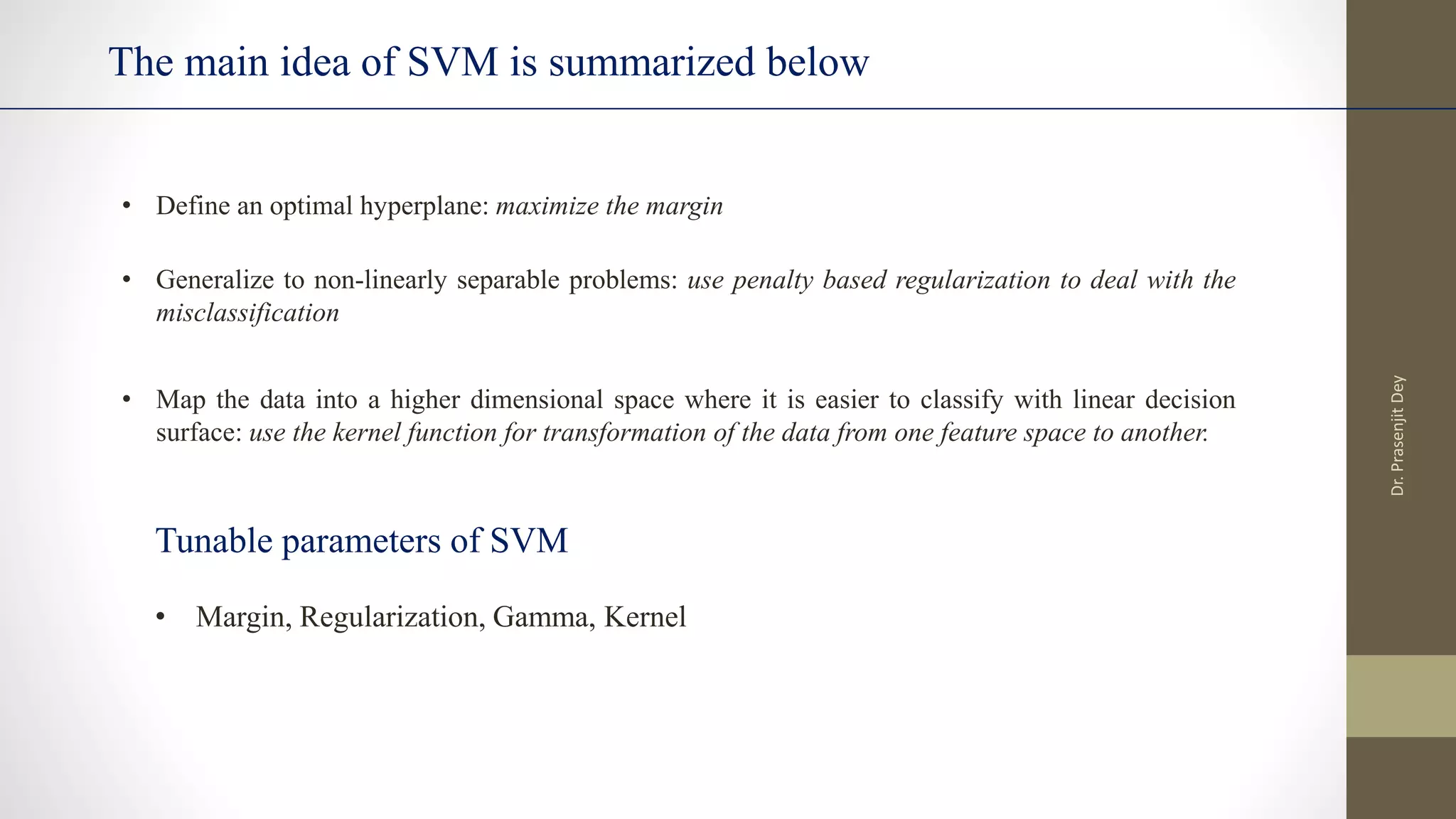
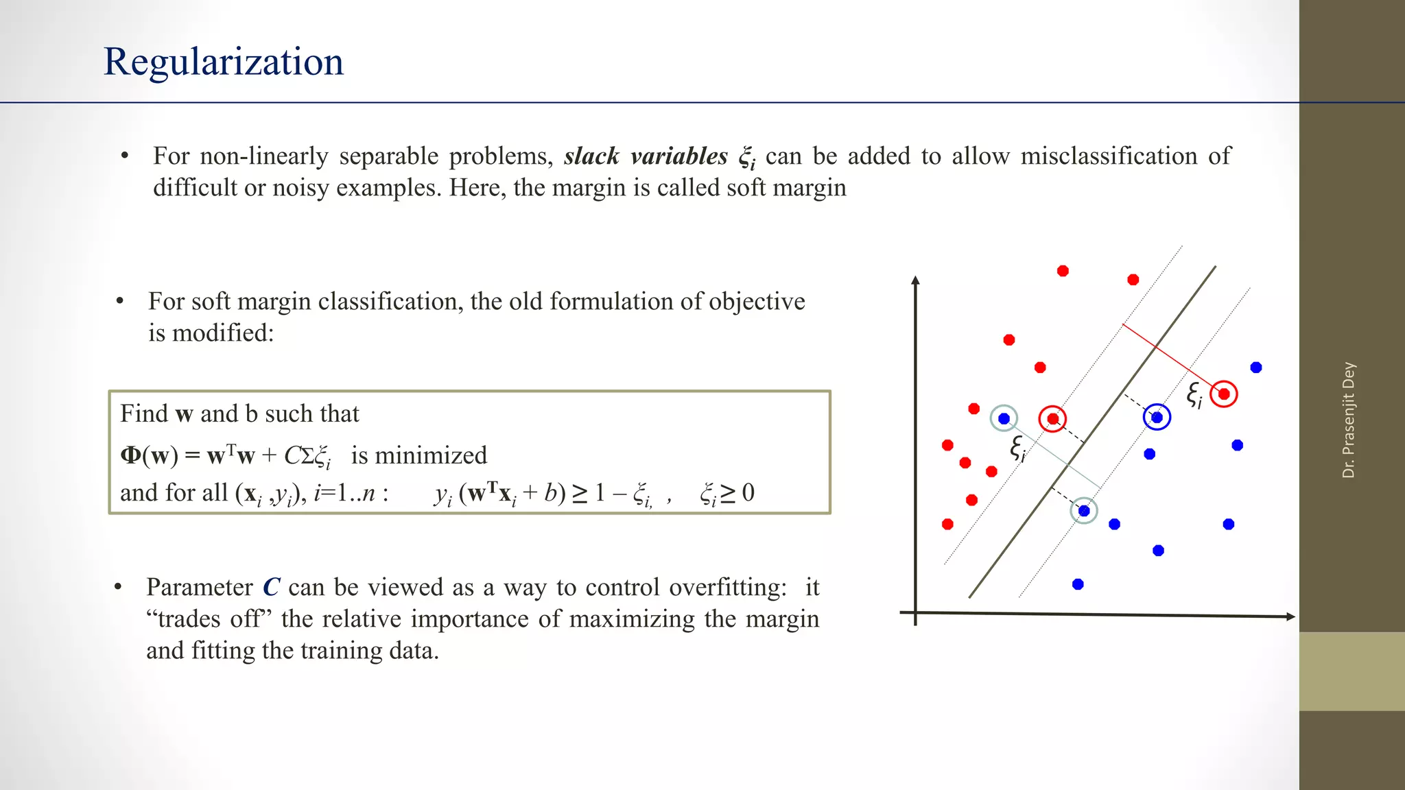
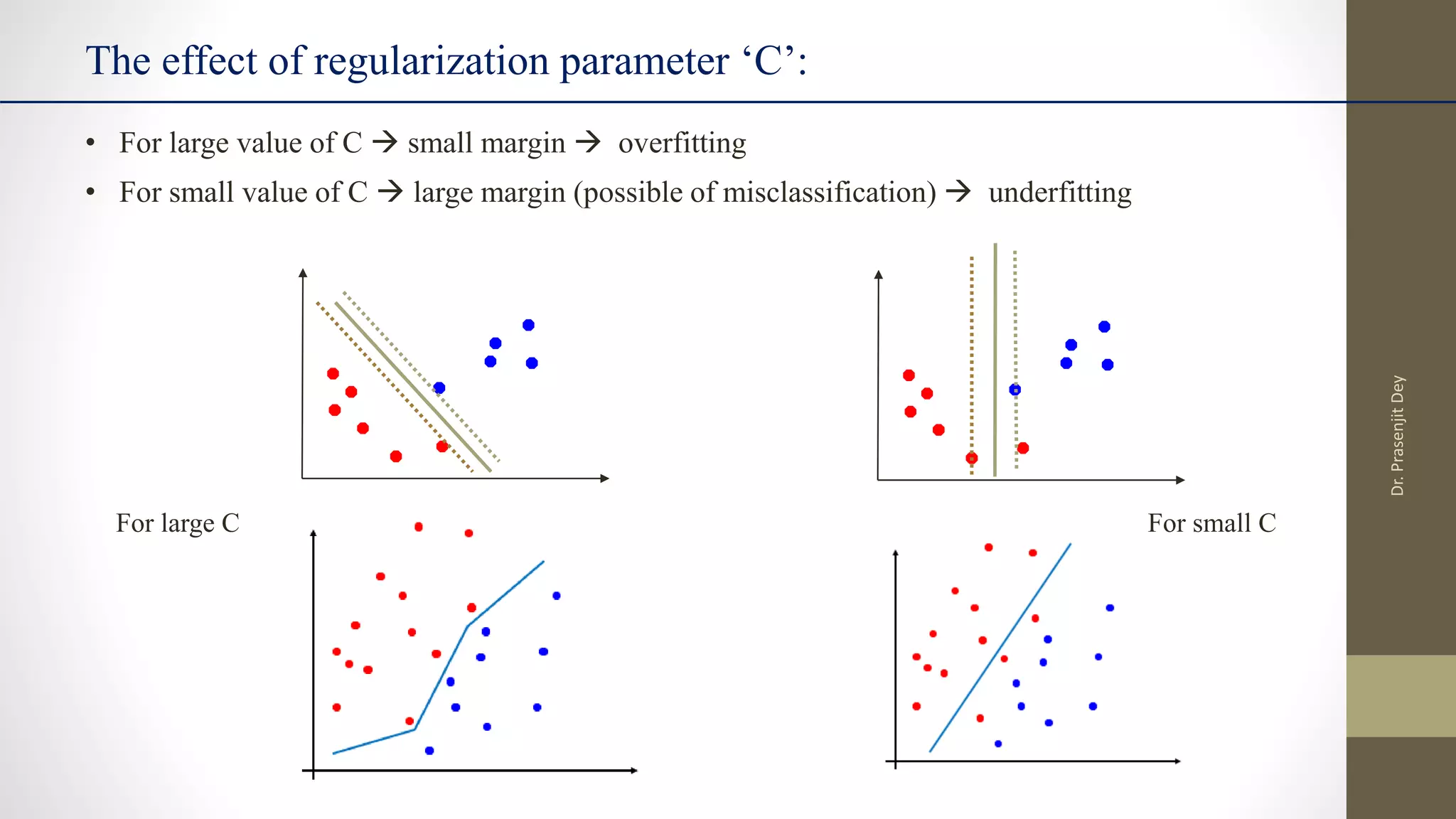
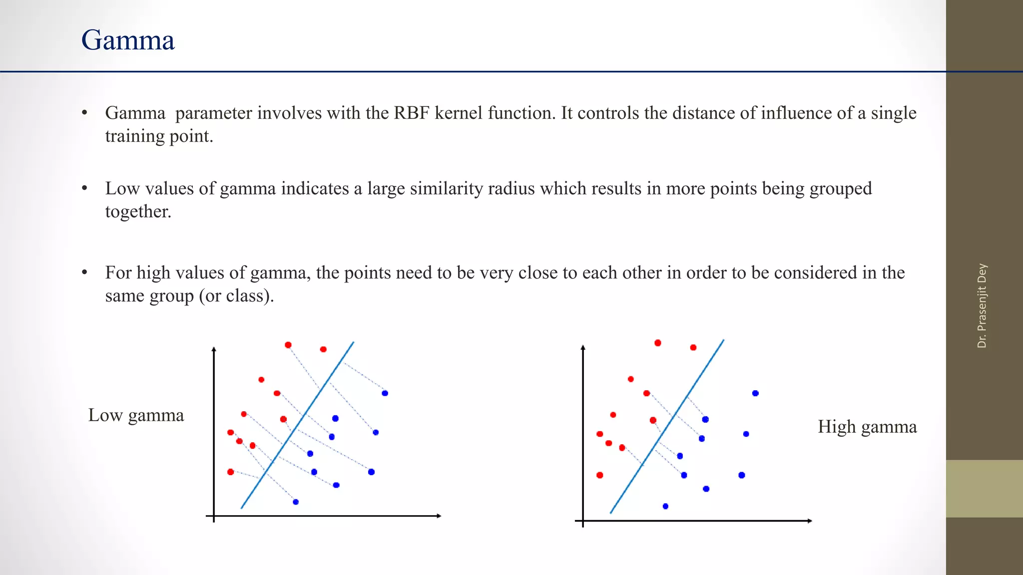
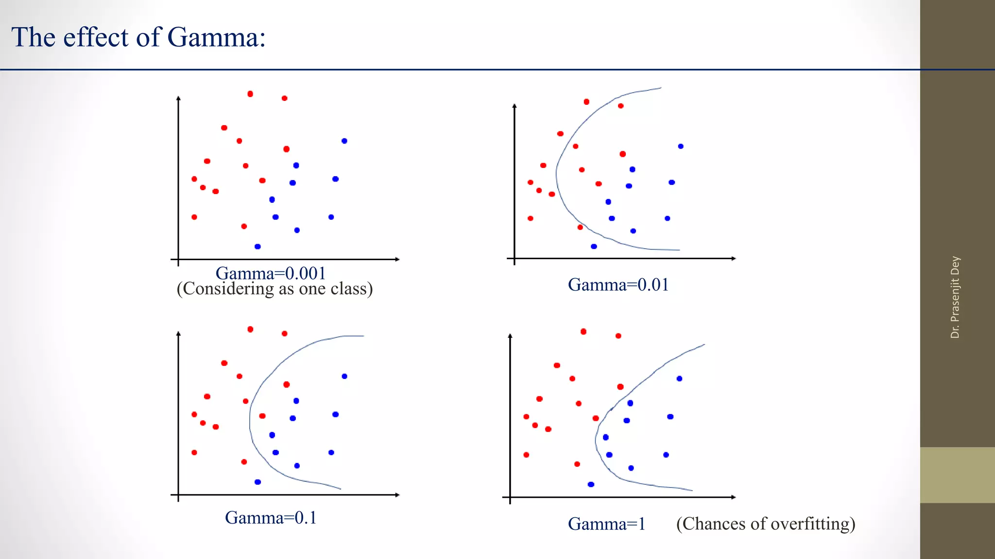


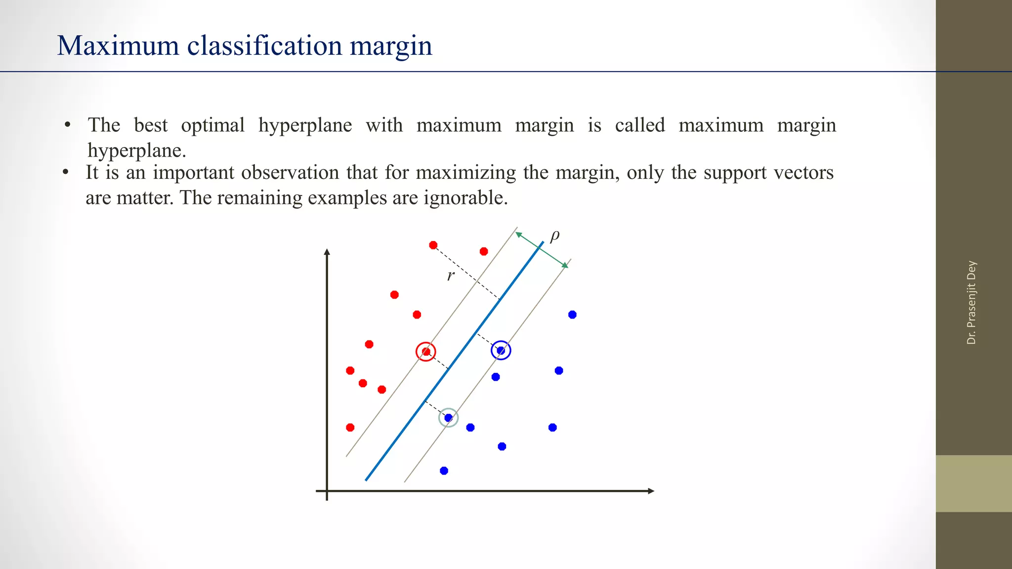
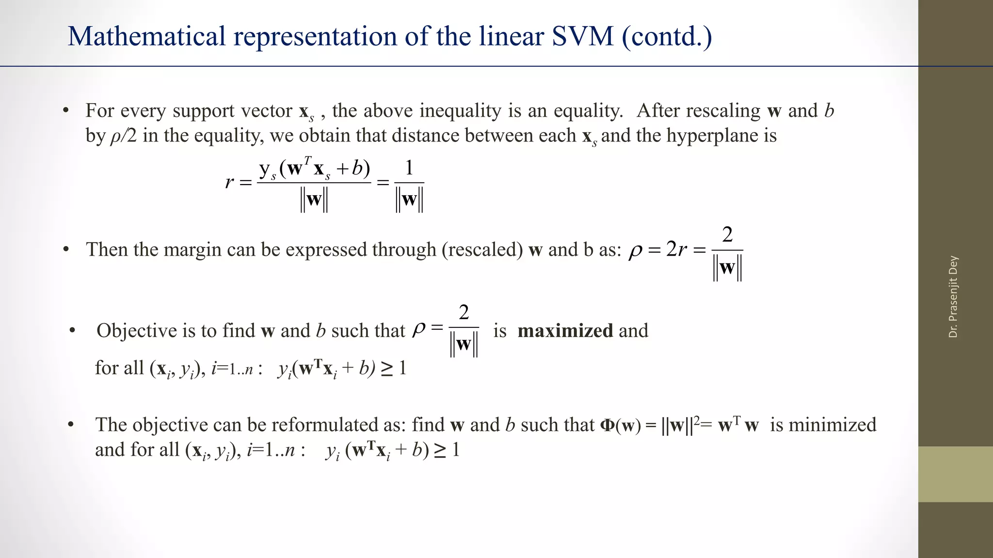
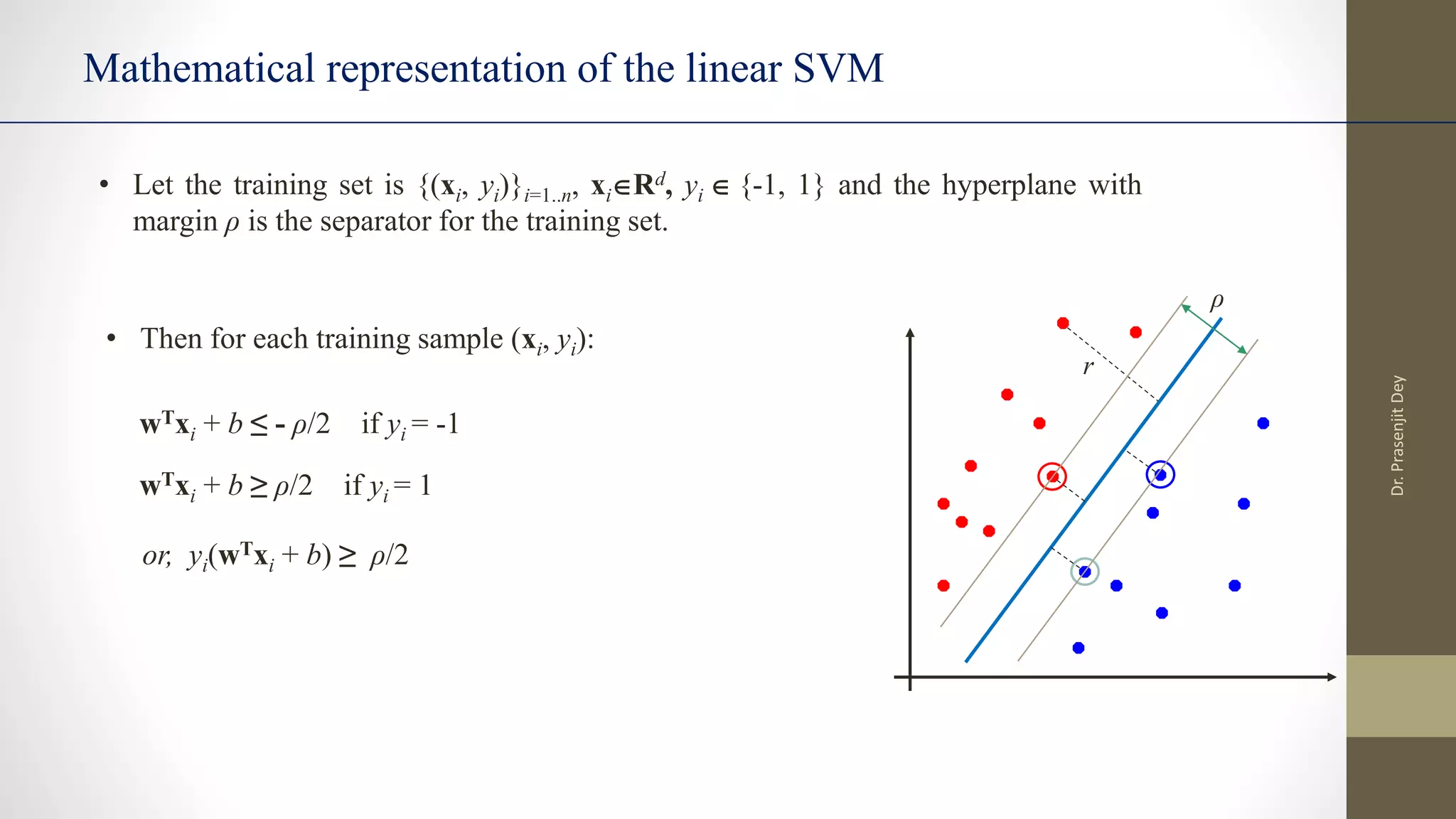
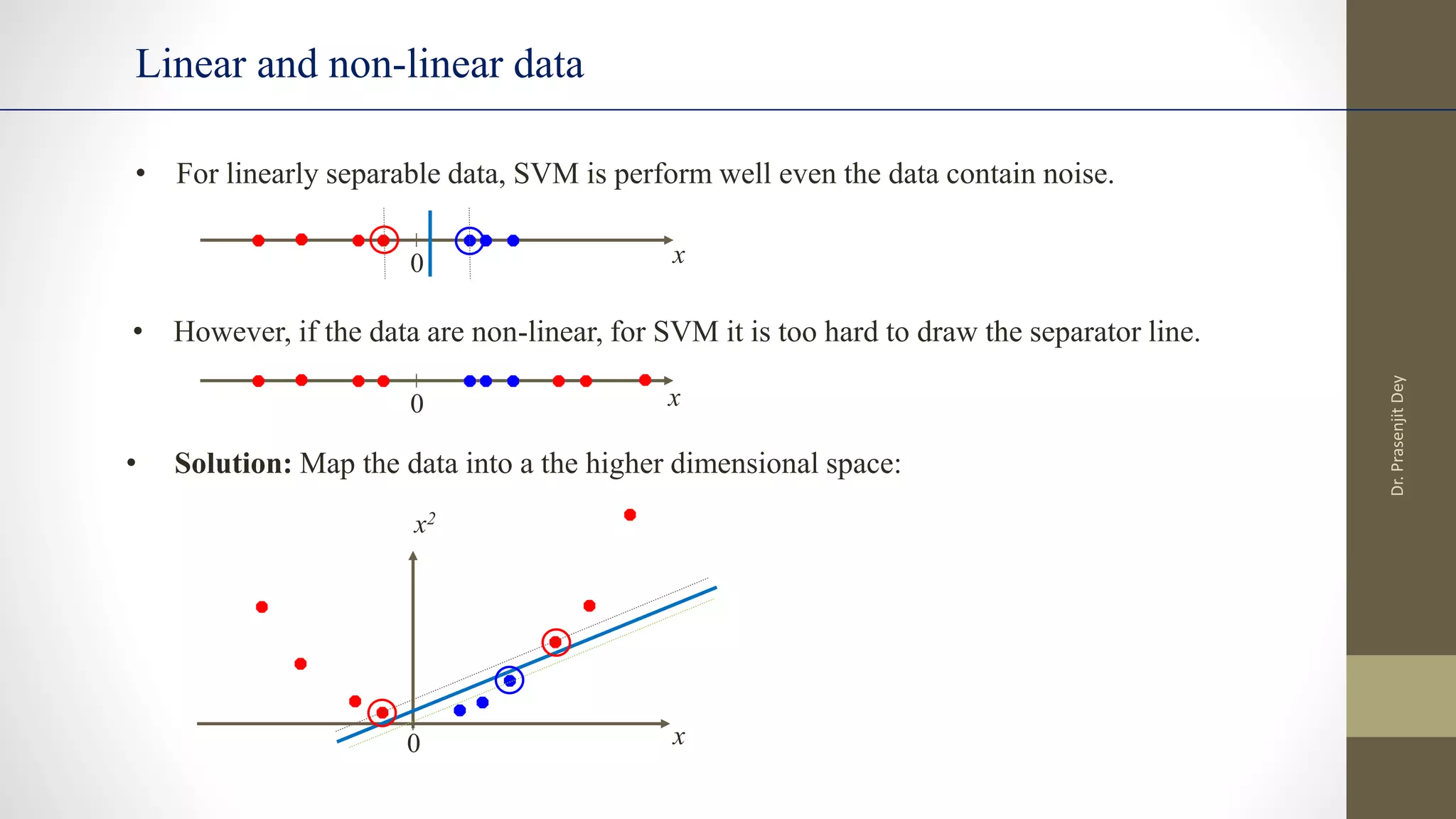
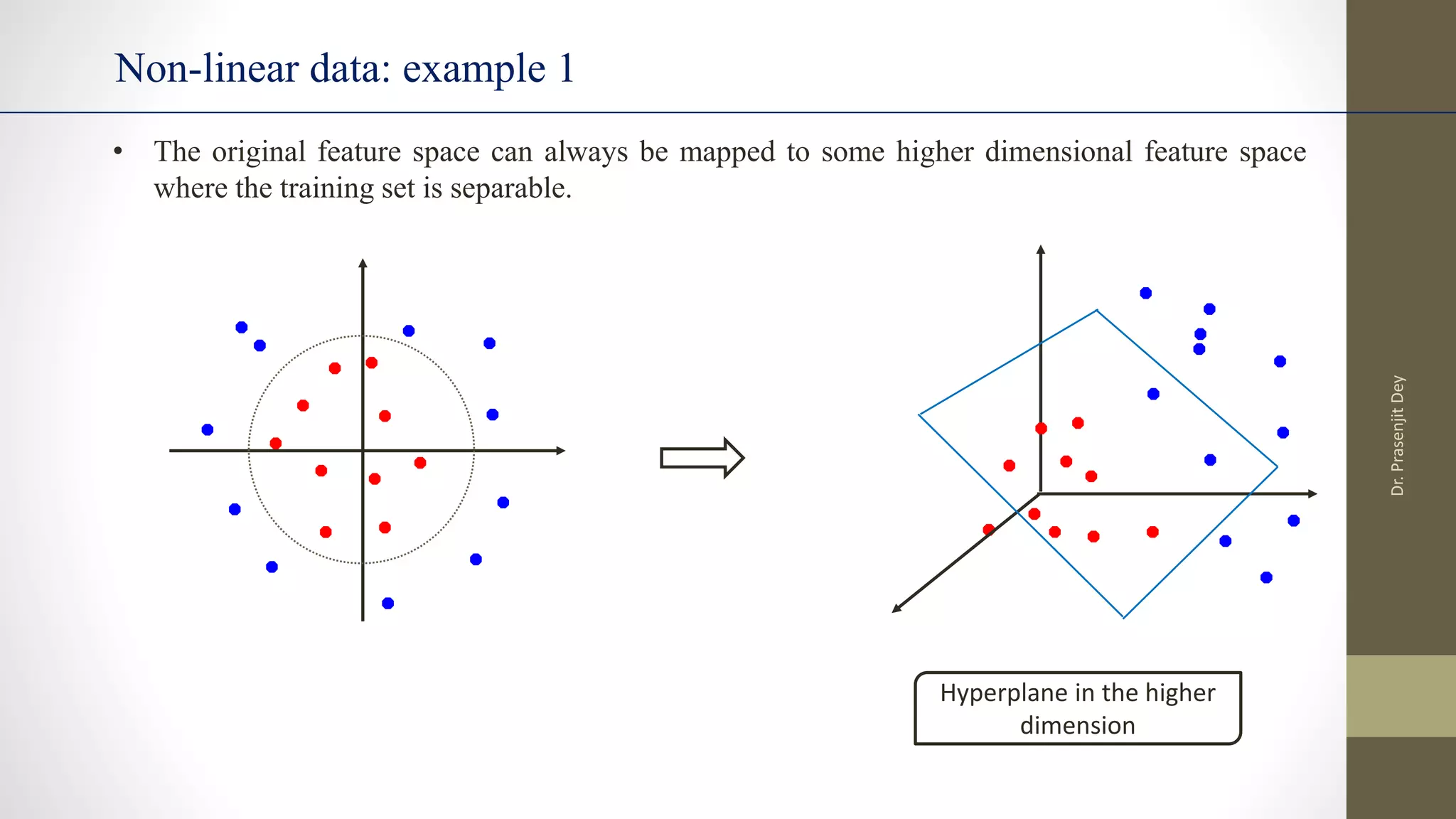
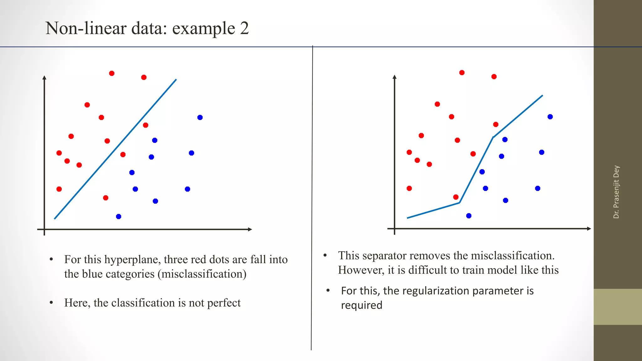
The document discusses support vector machines (SVMs). SVMs find the optimal separating hyperplane between classes that maximizes the margin between them. They can handle nonlinear data using kernels to map the data into higher dimensions where a linear separator may exist. Key aspects include defining the maximum margin hyperplane, using regularization and slack variables to deal with misclassified examples, and kernels which implicitly map data into other feature spaces without explicitly computing the transformations. The regularization and gamma parameters affect model complexity, with regularization controlling overfitting and gamma influencing the similarity between points.


![SVM[Support vector Machine] Machine learning](https://cdn.slidesharecdn.com/ss_thumbnails/svm-250403184638-1cd9afdb-thumbnail.jpg?width=640&height=640&fit=bounds)


![[DSC Europe 25] Dragana Ilic - AI for Big Data in Astronomy.pptx](https://cdn.slidesharecdn.com/ss_thumbnails/8palya86qaatvjhva1ms-2-dragana-ilic-ai-ilic-251208151906-652b819c-thumbnail.jpg?width=640&height=640&fit=bounds)
![[DSC Europe 25] Jovan Bogicevic - Legacy to AI-Driven Defense: Transforming D...](https://cdn.slidesharecdn.com/ss_thumbnails/rsarluadt563hntyfc8q-3-251211083849-3e7bc4c0-thumbnail.jpg?width=640&height=640&fit=bounds)
![[DSC Europe 25] Behzad Hosseini - AI Agents in the Wild: Deploying Models tha...](https://cdn.slidesharecdn.com/ss_thumbnails/3qtejajvsjqrzwfept2c-10-251212103250-7f2b1068-thumbnail.jpg?width=640&height=640&fit=bounds)
![[DSC Europe 25] Imai Jen-La Plante - The New Generation: AI and the Future of...](https://cdn.slidesharecdn.com/ss_thumbnails/kxi8t2l5rggivgcenyba-1-jenlaplante-dsc-251208152532-d1e076c2-thumbnail.jpg?width=640&height=640&fit=bounds)
![[DSC Europe 25] Sara Polak - The Ancient Operating System: What Archaeology T...](https://cdn.slidesharecdn.com/ss_thumbnails/3vch2p6tttdnwhsgazoz-3-sara-polak-smart-cities-251208152532-64404202-thumbnail.jpg?width=640&height=640&fit=bounds)

![[DSC Europe 25] Marija Vlajkovic & Andrea Radonjanin - Integration of AI tool...](https://cdn.slidesharecdn.com/ss_thumbnails/qf1jrglttoc3bm8s3aop-final-integration-of-ai-tools-251208151905-394f3a6a-thumbnail.jpg?width=640&height=640&fit=bounds)
![[DSC Europe 25] Branko Dzakula - From Defense to Attack: How AI Redefines Cyb...](https://cdn.slidesharecdn.com/ss_thumbnails/80bdzdxpr3ky2g0qvyk9-8-251211083048-ce5fc1ee-thumbnail.jpg?width=640&height=640&fit=bounds)


![[DSC Europe 25] Vladimir Jelic - The AI-Driven Security Shift From Reactive D...](https://cdn.slidesharecdn.com/ss_thumbnails/6g5gj25mtjwayniqem1t-6-251209104645-7a5a5fc6-thumbnail.jpg?width=640&height=640&fit=bounds)
![[DSC Europe 25] Dunja Adzic Jovanovic - AI and Cybersecurity: Defending Data ...](https://cdn.slidesharecdn.com/ss_thumbnails/o1zylpbhrtwnixxq2xj8-7-251211083048-185086f6-thumbnail.jpg?width=640&height=640&fit=bounds)
![[DSC Europe 25] Katherine Forrest - AI NOW: Understanding the Velocity of Cha...](https://cdn.slidesharecdn.com/ss_thumbnails/wvvbruqfrci0sfq9xwgb-4-251212104007-e5ad1987-thumbnail.jpg?width=640&height=640&fit=bounds)
![[DSC Europe 25] Milan Sekuloski - Data, Defence, and Development: Cybersecuri...](https://cdn.slidesharecdn.com/ss_thumbnails/dfrkwwx4qly6atqpbl4z-4-251209104645-c3d4b0ca-thumbnail.jpg?width=640&height=640&fit=bounds)
![[DSC Europe 25] Hans Kleinsman - The Compliance Gearbox: How Tax Tech Mediate...](https://cdn.slidesharecdn.com/ss_thumbnails/dxdytie1toel0hr90bjs-2-251212103250-174fdbe7-thumbnail.jpg?width=640&height=640&fit=bounds)