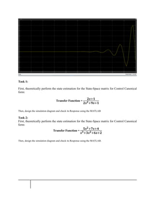
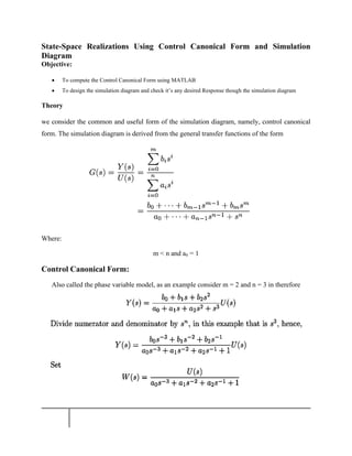
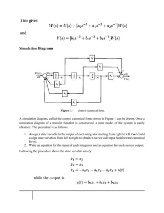
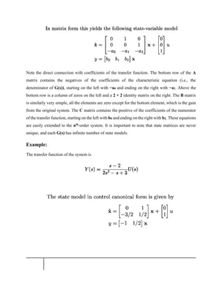
The document outlines an experiment for Avionics Engineering focusing on state-space realizations using control canonical form and simulation diagrams. It details the objectives and theoretical background necessary to compute the control canonical form with MATLAB, including the procedure to assign state variables and derive state matrices. The experiment includes two tasks that require theoretical state estimation and designing simulation diagrams to check system responses.

1. Department of Avionics Engineering
AE-3452
Modern Control Systems
Experiment No. 11
State-Space Realizations Using Control Canonical Form and
Simulation Diagram
Prepared for
By:
Name:
ID:
Section:
Semester:
Total Marks: ________________
Obtained Marks: _____________
Signature: __________________
Date: _____________________

2. State-Space Realizations Using Control Canonical Form and Simulation
Diagram
Objective:
• To compute the Control Canonical Form using MATLAB
• To design the simulation diagram and check it’s any desired Response though the simulation diagram
Theory
we consider the common and useful form of the simulation diagram, namely, control canonical
form. The simulation diagram is derived from the general transfer functions of the form
Where:
m < n and an = 1
Control Canonical Form:
Also called the phase variable model, as an example consider m = 2 and n = 3 in therefore

3. Simulation Diagrams
A simulation diagram, called the control canonical form shown in Figure 1 can be drawn. Once a
simulation diagram of a transfer function is constructed, a state model of the system is easily
obtained. The procedure is as follows:
1. Assign a state variable to the output of each integrator starting from right to left. (We could
assign state variables from left to right to obtain what we call input feedforward canonical
form).
2. Write an equation for the input of each integrator and an equation for each system output.
Following the procedure above the state variable satisfy:

4. Note the direct connection with coefficients of the transfer function. The bottom row of the A
matrix contains the negatives of the coefficients of the characteristic equation (i.e., the
denominator of G(s)), starting on the left with −a0 and ending on the right with −a2. Above the
bottom row is a column of zeros on the left and a 2 × 2 identity matrix on the right. The B matrix
is similarly very simple, all the elements are zero except for the bottom element, which is the gain
from the original system. The C matrix contains the positive of the coefficients of the numerator
of the transfer function, starting on the left with b0 and ending on the right with b2. These equations
are easily extended to the nth-order system. It is important to note that state matrices are never
unique, and each G(s) has infinite number of state models.
Example:
The transfer function of the system is

5. CODE:
Num=[1 -2];
Dem=[2 -1 3];
sys=tf(Num,Dem)
[A,B,C,D]=tf2ss(Num,Dem)
Simulation Diagram:
Same
Response:

6. Task 1:
First, theoretically perform the state estimation for the State-Space matrix for Control Canonical
form:
Transfer Function =
𝟐𝒔+𝟏
𝟐𝒔𝟐+𝟗𝒔+𝟏
Then, design the simulation diagram and check its Response using the MATLAB
Task 2:
First, theoretically perform the state estimation for the State-Space matrix for Control Canonical
form:
Transfer Function =
𝟓𝒔𝟐+𝟕𝒔+𝟒
𝒔𝟑+𝟑𝒔𝟐+𝟔𝒔+𝟐
Then, design the simulation diagram and check its Response using the MATLAB.