Mathematical Modeling ofDynamic Systems
• Outline
– Review of Classical Control Systems
• Transfer Function (3.2)
• Block Diagram and Mason’s Gain Formula(3.3)
– State Variable Modeling (3.4)
3.
State Variable Modeling
•State
– The smallest set of variables, called state variables such that the
knowledge of these variables at t = 𝑡𝑡0, together with the knowledge
of input for 𝑡𝑡 < 𝑡𝑡0, determines the system behavior for 𝑡𝑡 ≥ 𝑡𝑡0
• State Variable
– The variables that determine the state of the dynamic
system,𝑥𝑥1, 𝑥𝑥2, … , 𝑥𝑥𝑛𝑛. The number of state variables is dependent on
the order of the system, number of inputs and outputs.
• State Vector
– If n variables 𝑥𝑥1, 𝑥𝑥2, … , 𝑥𝑥𝑛𝑛 describe the system, then these 𝑛𝑛 variables
are considered as the n-components of a vector 𝑥𝑥(𝑡𝑡). This vector is
called the state vector
𝑥𝑥 𝑡𝑡 =
𝑥𝑥1
⋮
𝑥𝑥𝑛𝑛
4.
More Definitions
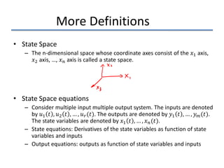
• StateSpace
– The n-dimensional space whose coordinate axes consist of the 𝑥𝑥1 axis,
𝑥𝑥2 axis, …, 𝑥𝑥𝑛𝑛 axis is called a state space.
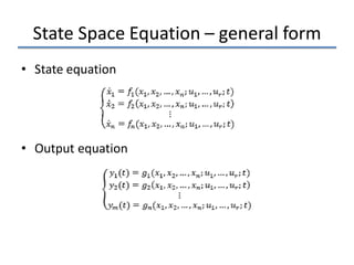
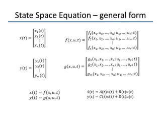
• State Space equations
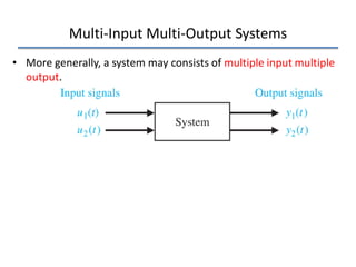
– Consider multiple input multiple output system. The inputs are denoted
by 𝑢𝑢1 𝑡𝑡 , 𝑢𝑢2 𝑡𝑡 , … , 𝑢𝑢𝑟𝑟(𝑡𝑡). The outputs are denoted by 𝑦𝑦1 𝑡𝑡 , … , 𝑦𝑦𝑚𝑚(𝑡𝑡).
The state variables are denoted by 𝑥𝑥1 𝑡𝑡 , … , 𝑥𝑥𝑛𝑛(𝑡𝑡).
– State equations: Derivatives of the state variables as function of state
variables and inputs
– Output equations: outputs as function of state variables and inputs
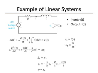
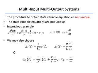
Multi-Input Multi-Output Systems
•The procedure to obtain state variable equations is not unique
• The state variable equations are not unique
• In previous example
• We may also choose
𝑥𝑥1 𝑡𝑡 =
1
𝐿𝐿𝐿𝐿
𝑖𝑖 𝑡𝑡 , 𝑥𝑥2 𝑡𝑡 =
𝑅𝑅
𝐿𝐿
𝑑𝑑𝑑𝑑
𝑑𝑑𝑑𝑑
Or
𝑥𝑥1 𝑡𝑡 =
1
𝐿𝐿𝐿𝐿
𝑖𝑖 𝑡𝑡 +
𝑅𝑅
𝐿𝐿
𝑑𝑑𝑑𝑑
𝑑𝑑𝑑𝑑
, 𝑥𝑥2 =
𝑑𝑑𝑑𝑑
𝑑𝑑𝑑𝑑
Multi-Input Multi-Output Systems(Cont.)
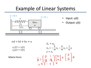
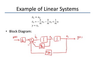
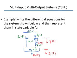
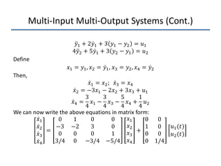
• Example: write the differential equations for
the system shown below and then represent
them in state variable form
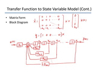
Transfer Function toState Variable Models
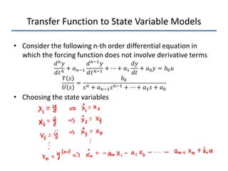
• Consider the following n-th order differential equation in
which the forcing function does not involve derivative terms
𝑑𝑑𝑛𝑛𝑦𝑦
𝑑𝑑𝑡𝑡𝑛𝑛
+ 𝑎𝑎𝑛𝑛−1
𝑑𝑑𝑛𝑛−1𝑦𝑦
𝑑𝑑𝑡𝑡𝑛𝑛−1
+ ⋯ + 𝑎𝑎1
𝑑𝑑𝑦𝑦
𝑑𝑑𝑡𝑡
+ 𝑎𝑎0𝑦𝑦 = 𝑏𝑏0𝑢𝑢
𝑌𝑌 𝑠𝑠
𝑈𝑈 𝑠𝑠
=
𝑏𝑏0
𝑠𝑠𝑛𝑛 + 𝑎𝑎𝑛𝑛−1𝑠𝑠𝑛𝑛−1 + ⋯ + 𝑎𝑎1𝑠𝑠 + 𝑎𝑎0
• Choosing the state variables
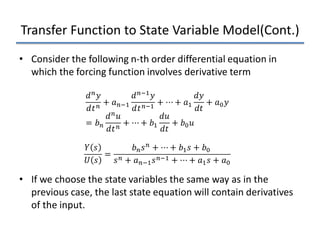
Transfer Function toState Variable Model(Cont.)
• Consider the following n-th order differential equation in
which the forcing function involves derivative term
• If we choose the state variables the same way as in the
previous case, the last state equation will contain derivatives
of the input.
𝑑𝑑𝑛𝑛𝑦𝑦
𝑑𝑑𝑡𝑡𝑛𝑛
+ 𝑎𝑎𝑛𝑛−1
𝑑𝑑𝑛𝑛−1𝑦𝑦
𝑑𝑑𝑡𝑡𝑛𝑛−1
+ ⋯ + 𝑎𝑎1
𝑑𝑑𝑑𝑑
𝑑𝑑𝑑𝑑
+ 𝑎𝑎0𝑦𝑦
= 𝑏𝑏𝑛𝑛
𝑑𝑑𝑛𝑛𝑢𝑢
𝑑𝑑𝑡𝑡𝑛𝑛
+ ⋯ + 𝑏𝑏1
𝑑𝑑𝑢𝑢
𝑑𝑑𝑑𝑑
+ 𝑏𝑏0𝑢𝑢
𝑌𝑌 𝑠𝑠
𝑈𝑈 𝑠𝑠
=
𝑏𝑏𝑛𝑛𝑠𝑠𝑛𝑛 + ⋯ + 𝑏𝑏1𝑠𝑠 + 𝑏𝑏0
𝑠𝑠𝑛𝑛 + 𝑎𝑎𝑛𝑛−1𝑠𝑠𝑛𝑛−1 + ⋯ + 𝑎𝑎1𝑠𝑠 + 𝑎𝑎0
19.
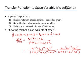
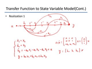
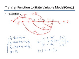
Transfer Function toState Variable Model(Cont.)
• A general approach:
1) Realize system in block diagram or signal flow graph
2) Name the integrator output as state variables
3) Write the equations for inputs of integrators
• Show the method on an example of order 3
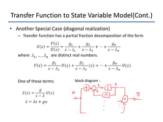
Transfer Function toState Variable Model(Cont.)
• Another Special Case (diagonal realization)
– Transfer function has a partial fraction decomposition of the form
where are distinct real numbers.
One of these terms: block diagram :