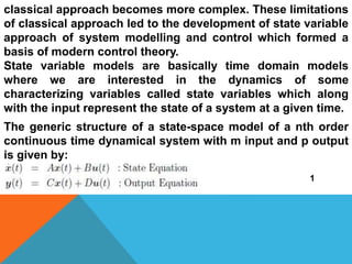
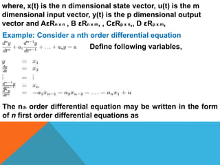
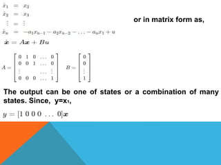
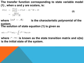
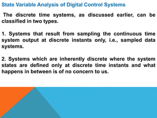
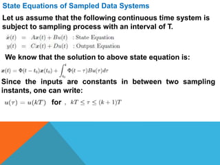
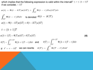
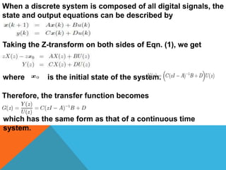
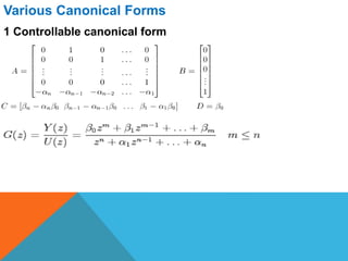
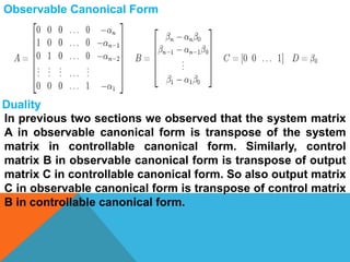
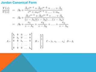
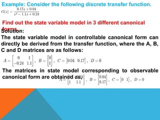
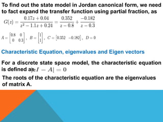
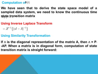
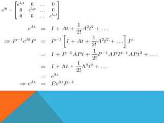
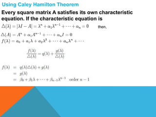
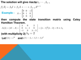
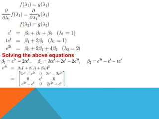
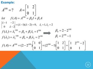
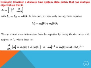
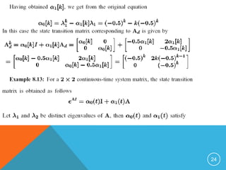
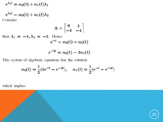
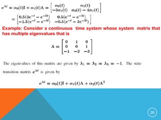
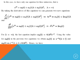
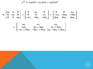
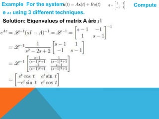
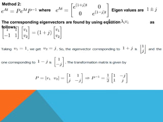
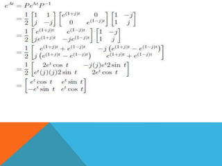
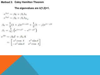
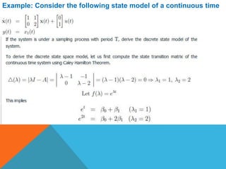
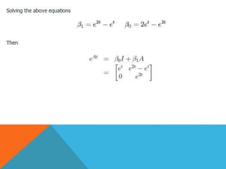
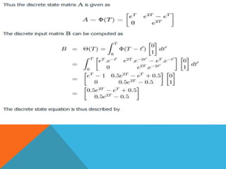
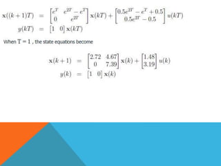
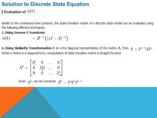
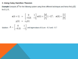
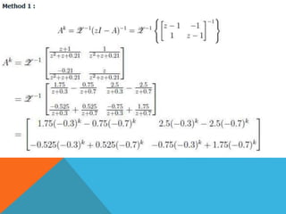
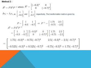
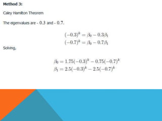
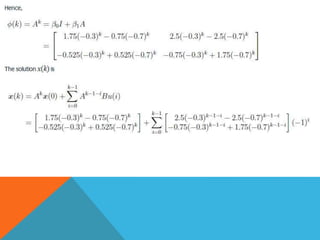
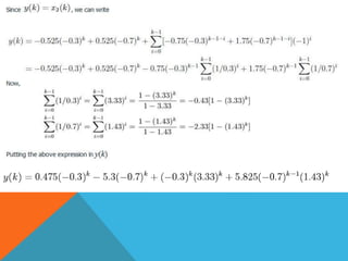
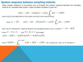
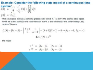
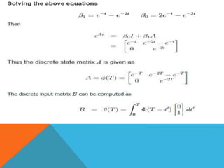
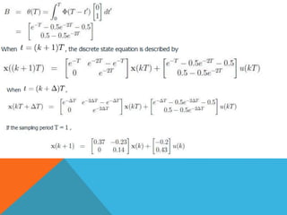
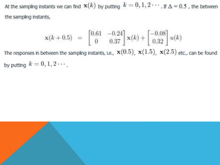
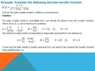
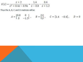
Assist. Prof. Dr. Khalaf S. Gaeid
Electrical Engineering Department
Tikrit University
gaeidkhalaf@gmail.com
+9647703057076
Discrete state space model
1. Introduction to state variable model
2. Various canonical forms
3. Characteristic equation
4. state transition matrix
5. Solution to discrete state equation
6.Examples
Contents
Introduction to State Variable Model
In the preceding lectures, we have learned how to design a
sampled data control system or a digital system using the
transfer function of the system to be controlled. Transfer
function approach of system modelling provides final relation
between output variable and input variable.
However, a system may have other internal variables of
importance. State variable representation takes into account
of all such internal variables. Moreover, controller design
using classical methods, e.g., root locus or frequency domain
method are limited to only LTI systems, particularly SISO
(single input single output) systems since for MIMO (multi
input multi output) systems controller design using
classical approach becomes more complex. These limitations
of classical approach led to the development of state variable
approach of system modelling and control which formed a
basis of modern control theory.
State variable models are basically time domain models
where we are interested in the dynamics of some
characterizing variables called state variables which along
with the input represent the state of a system at a given time.
The generic structure of a state-space model of a nth order
continuous time dynamical system with m input and p output
is given by:
1
where, x(t) is the n dimensional state vector, u(t) is the m
dimensional input vector, y(t) is the p dimensional output
vector and AεRn x n , B εRn x m, , CεRp x n,, D εRp x m,
Example: Consider a nth order differential equation
Define following variables,
The nth order differential equation may be written in the form
of n first order differential equations as
or in matrix form as,
The output can be one of states or a combination of many
states. Since, y=x1,
The transfer function corresponding to state variable model
(1) , when u and y are scalars, is:
(2)
where is the characteristic polynomial of the
system.
The solution of state equation (1) is given as
where is known as the state transition matrix and x(to)
is the initial state of the system.
State Variable Analysis of Digital Control Systems
The discrete time systems, as discussed earlier, can be
classified in two types.
1. Systems that result from sampling the continuous time
system output at discrete instants only, i.e., sampled data
systems.
2. Systems which are inherently discrete where the system
states are defined only at discrete time instants and what
happens in between is of no concern to us.
State Equations of Sampled Data Systems
Let us assume that the following continuous time system is
subject to sampling process with an interval of T.
We know that the solution to above state equation is:
Since the inputs are constants in between two sampling
instants, one can write:
for
which implies that the following expression is valid within the interval
if we consider
Is denoted
(4)
and
If we can rewrite
When a discrete system is composed of all digital signals, the
state and output equations can be described by
Taking the Z-transform on both sides of Eqn. (1), we get
where is the initial state of the system.
Therefore, the transfer function becomes
which has the same form as that of a continuous time
system.
Various Canonical Forms
1 Controllable canonical form
Observable Canonical Form
Duality
In previous two sections we observed that the system matrix
A in observable canonical form is transpose of the system
matrix in controllable canonical form. Similarly, control
matrix B in observable canonical form is transpose of output
matrix C in controllable canonical form. So also output matrix
C in observable canonical form is transpose of control matrix
B in controllable canonical form.
Jordan Canonical Form
Example: Consider the following discrete transfer function.
Find out the state variable model in 3 different canonical
forms.Solution:
The state variable model in controllable canonical form can
directly be derived from the transfer function, where the A, B,
C and D matrices are as follows:
The matrices in state model corresponding to observable
canonical form are obtained as,
To find out the state model in Jordan canonical form, we need
to fact expand the transfer function using partial fraction, as
Characteristic Equation, eigenvalues and Eigen vectors
For a discrete state space model, the characteristic equation
is defined as
The roots of the characteristic equation are the eigenvalues
of matrix A.
Computation of
We have seen that to derive the state space model of a
sampled data system, we need to know the continuous time
state transition matrix
Using Inverse Laplace Transform
Using Similarity Transformation
If ∧ is the diagonal representation of the matrix A, then ∧ = P-
1AP. When a matrix is in diagonal form, computation of state
transition matrix is straight forward:
Using Caley Hamilton Theorem
Every square matrix A satisfies its own characteristic
equation. If the characteristic equation is
then,
The solution will give rise to
Example :
then compute the state transition matrix using Caley
Hamilton Theorem.
(with multiplicity 2)
Let and
Solving the above equations
22







10
21
?100
AA
Example:
AIAAflet 10
100
)(  
2,1,0)2)(1(
20
21
21 





100
210
100
22
100
110
100
11
2)(
1)(




f
f
12
22
100
1
100
0









 













10
221
10
21
)12(
10
01
)22()(
101
100100100
AAf
23
Example: Consider a discrete time system state matrix that has multiple
eigenvalues that is
24
25
26
Example: Consider a continuous time system whose system matrix that
has multiple eigenvalues that is
27
28
Example For the system Compute
e A t using 3 different techniques.
Solution: Eigenvalues of matrix A are
Method 2:
where Eigen values are
The corresponding eigenvectors are found by using equation as
follows:
Method 3: Caley Hamilton Theorem
The eigenvalues are λ{1,2}=1.
Example: Consider the following state model of a continuous time
system.
Solution to Discrete State Equation
System response between sampling instants
Example: Consider the following state model of a continuous time
system
Example: Consider the following discrete transfer function
Thanks

Discrete state space model 9th &10th lecture

  • 1.
    Assist. Prof. Dr.Khalaf S. Gaeid Electrical Engineering Department Tikrit University gaeidkhalaf@gmail.com +9647703057076 Discrete state space model
  • 2.
    1. Introduction tostate variable model 2. Various canonical forms 3. Characteristic equation 4. state transition matrix 5. Solution to discrete state equation 6.Examples Contents
  • 3.
    Introduction to StateVariable Model In the preceding lectures, we have learned how to design a sampled data control system or a digital system using the transfer function of the system to be controlled. Transfer function approach of system modelling provides final relation between output variable and input variable. However, a system may have other internal variables of importance. State variable representation takes into account of all such internal variables. Moreover, controller design using classical methods, e.g., root locus or frequency domain method are limited to only LTI systems, particularly SISO (single input single output) systems since for MIMO (multi input multi output) systems controller design using
  • 4.
    classical approach becomesmore complex. These limitations of classical approach led to the development of state variable approach of system modelling and control which formed a basis of modern control theory. State variable models are basically time domain models where we are interested in the dynamics of some characterizing variables called state variables which along with the input represent the state of a system at a given time. The generic structure of a state-space model of a nth order continuous time dynamical system with m input and p output is given by: 1
  • 5.
    where, x(t) isthe n dimensional state vector, u(t) is the m dimensional input vector, y(t) is the p dimensional output vector and AεRn x n , B εRn x m, , CεRp x n,, D εRp x m, Example: Consider a nth order differential equation Define following variables, The nth order differential equation may be written in the form of n first order differential equations as
  • 6.
    or in matrixform as, The output can be one of states or a combination of many states. Since, y=x1,
  • 7.
    The transfer functioncorresponding to state variable model (1) , when u and y are scalars, is: (2) where is the characteristic polynomial of the system. The solution of state equation (1) is given as where is known as the state transition matrix and x(to) is the initial state of the system.
  • 8.
    State Variable Analysisof Digital Control Systems The discrete time systems, as discussed earlier, can be classified in two types. 1. Systems that result from sampling the continuous time system output at discrete instants only, i.e., sampled data systems. 2. Systems which are inherently discrete where the system states are defined only at discrete time instants and what happens in between is of no concern to us.
  • 9.
    State Equations ofSampled Data Systems Let us assume that the following continuous time system is subject to sampling process with an interval of T. We know that the solution to above state equation is: Since the inputs are constants in between two sampling instants, one can write: for
  • 10.
    which implies thatthe following expression is valid within the interval if we consider Is denoted (4) and If we can rewrite
  • 11.
    When a discretesystem is composed of all digital signals, the state and output equations can be described by Taking the Z-transform on both sides of Eqn. (1), we get where is the initial state of the system. Therefore, the transfer function becomes which has the same form as that of a continuous time system.
  • 12.
    Various Canonical Forms 1Controllable canonical form
  • 13.
    Observable Canonical Form Duality Inprevious two sections we observed that the system matrix A in observable canonical form is transpose of the system matrix in controllable canonical form. Similarly, control matrix B in observable canonical form is transpose of output matrix C in controllable canonical form. So also output matrix C in observable canonical form is transpose of control matrix B in controllable canonical form.
  • 14.
  • 15.
    Example: Consider thefollowing discrete transfer function. Find out the state variable model in 3 different canonical forms.Solution: The state variable model in controllable canonical form can directly be derived from the transfer function, where the A, B, C and D matrices are as follows: The matrices in state model corresponding to observable canonical form are obtained as,
  • 16.
    To find outthe state model in Jordan canonical form, we need to fact expand the transfer function using partial fraction, as Characteristic Equation, eigenvalues and Eigen vectors For a discrete state space model, the characteristic equation is defined as The roots of the characteristic equation are the eigenvalues of matrix A.
  • 17.
    Computation of We haveseen that to derive the state space model of a sampled data system, we need to know the continuous time state transition matrix Using Inverse Laplace Transform Using Similarity Transformation If ∧ is the diagonal representation of the matrix A, then ∧ = P- 1AP. When a matrix is in diagonal form, computation of state transition matrix is straight forward:
  • 19.
    Using Caley HamiltonTheorem Every square matrix A satisfies its own characteristic equation. If the characteristic equation is then,
  • 20.
    The solution willgive rise to Example : then compute the state transition matrix using Caley Hamilton Theorem. (with multiplicity 2) Let and
  • 21.
  • 22.
    22        10 21 ?100 AA Example: AIAAflet 10 100 )(  2,1,0)2)(1( 20 21 21       100 210 100 22 100 110 100 11 2)( 1)(     f f 12 22 100 1 100 0                         10 221 10 21 )12( 10 01 )22()( 101 100100100 AAf
  • 23.
    23 Example: Consider adiscrete time system state matrix that has multiple eigenvalues that is
  • 24.
  • 25.
  • 26.
    26 Example: Consider acontinuous time system whose system matrix that has multiple eigenvalues that is
  • 27.
  • 28.
  • 29.
    Example For thesystem Compute e A t using 3 different techniques. Solution: Eigenvalues of matrix A are
  • 30.
    Method 2: where Eigenvalues are The corresponding eigenvectors are found by using equation as follows:
  • 32.
    Method 3: CaleyHamilton Theorem The eigenvalues are λ{1,2}=1.
  • 33.
    Example: Consider thefollowing state model of a continuous time system.
  • 37.
    Solution to DiscreteState Equation
  • 44.
    System response betweensampling instants
  • 45.
    Example: Consider thefollowing state model of a continuous time system
  • 49.
    Example: Consider thefollowing discrete transfer function
  • 51.