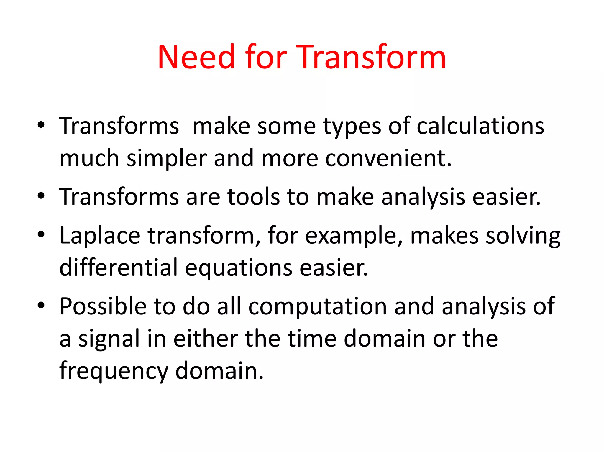
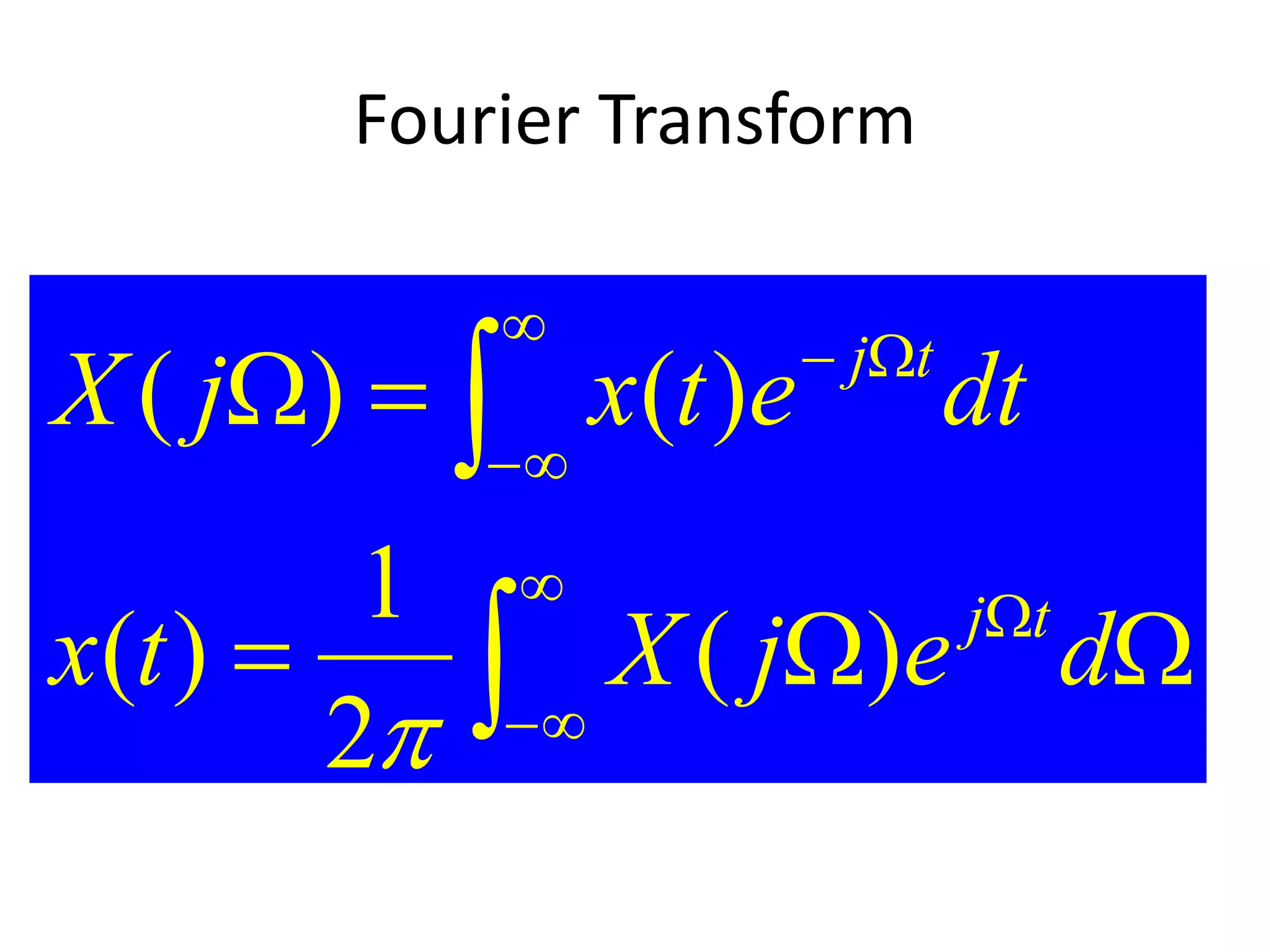
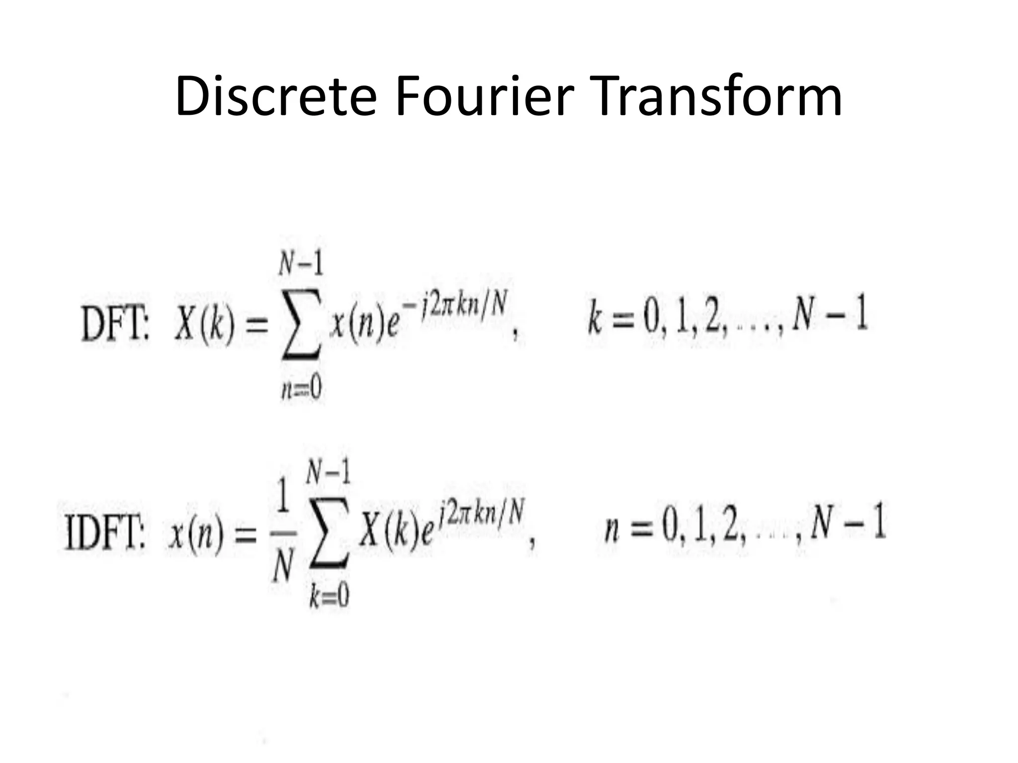
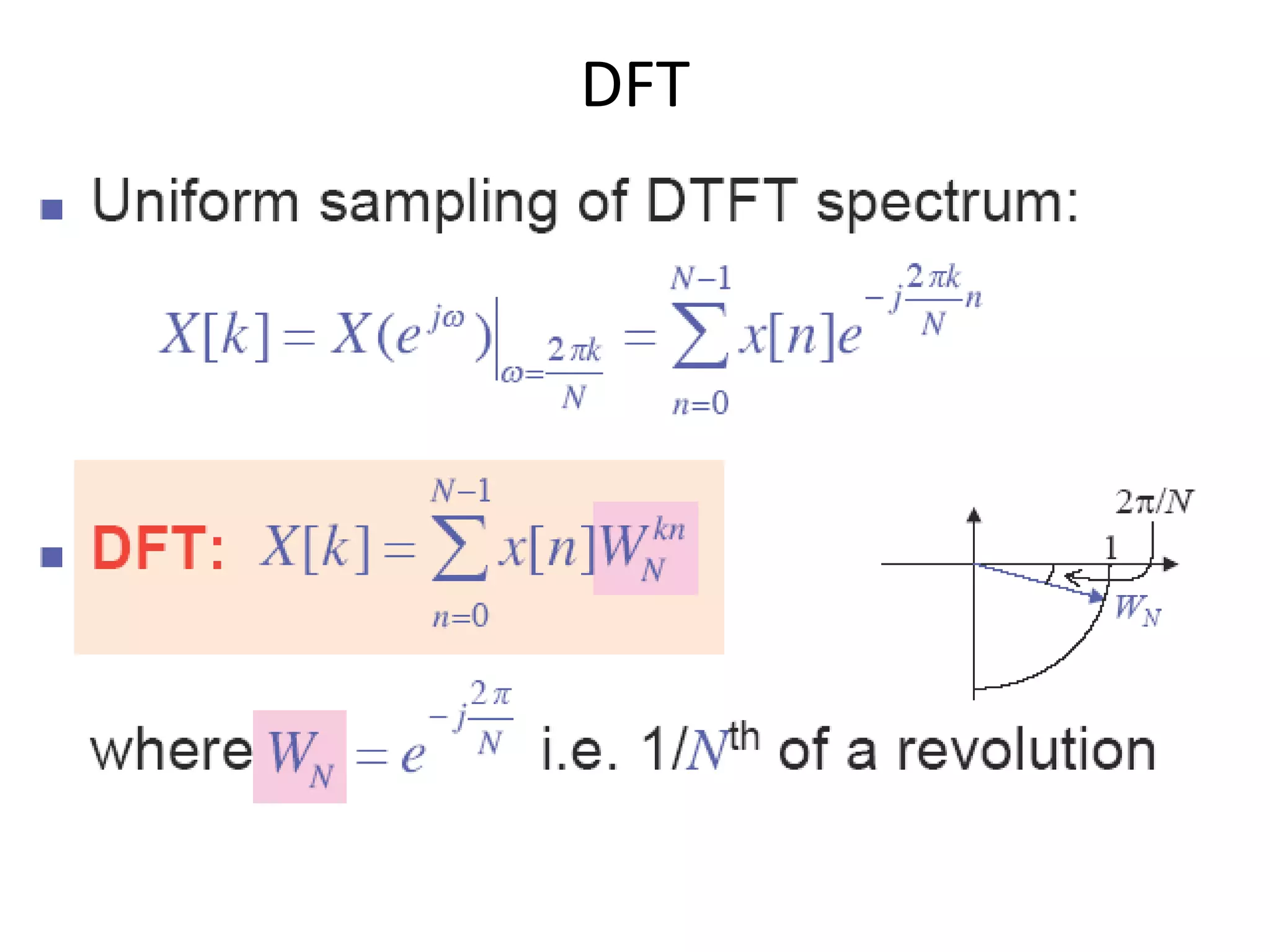
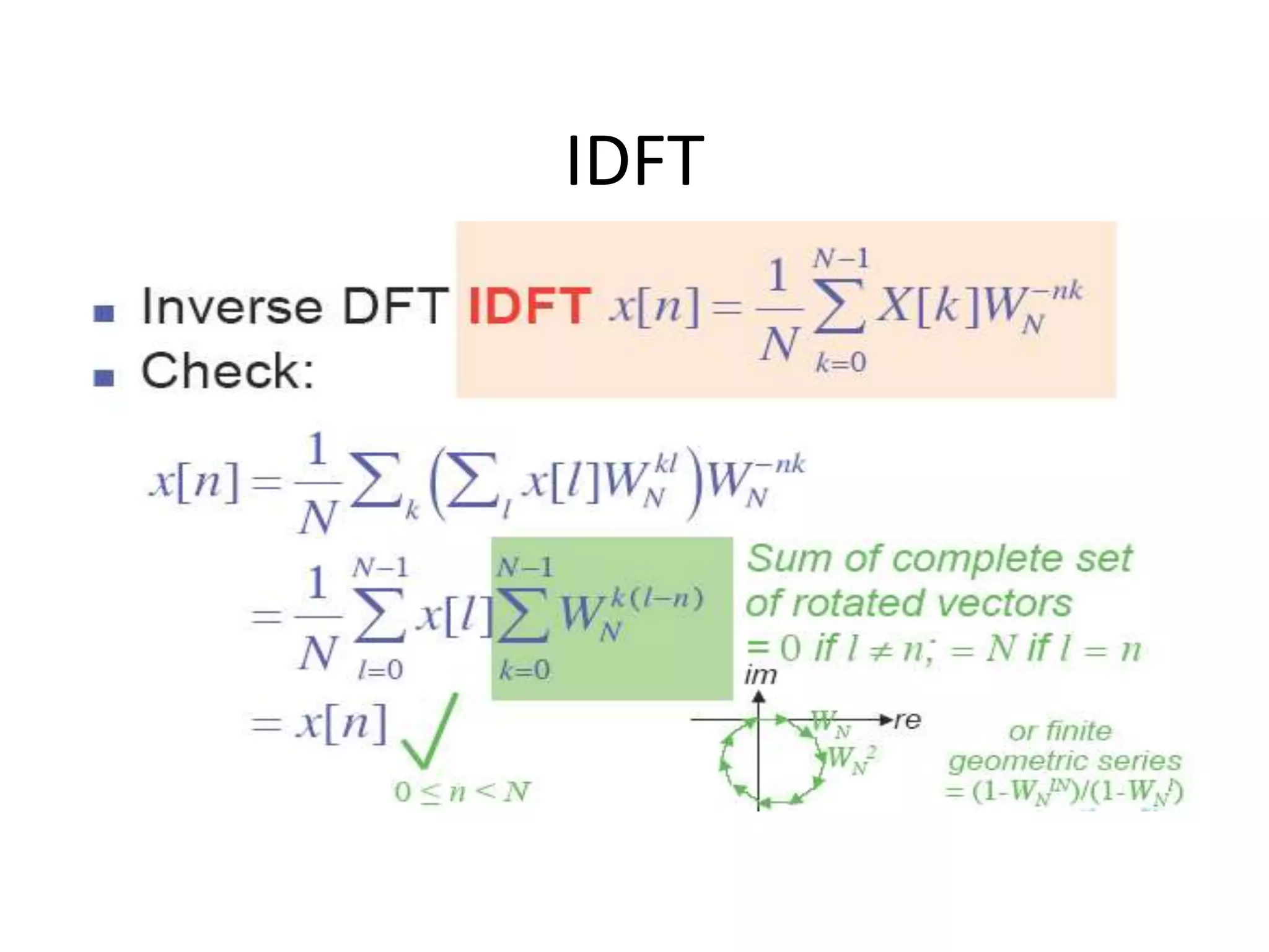
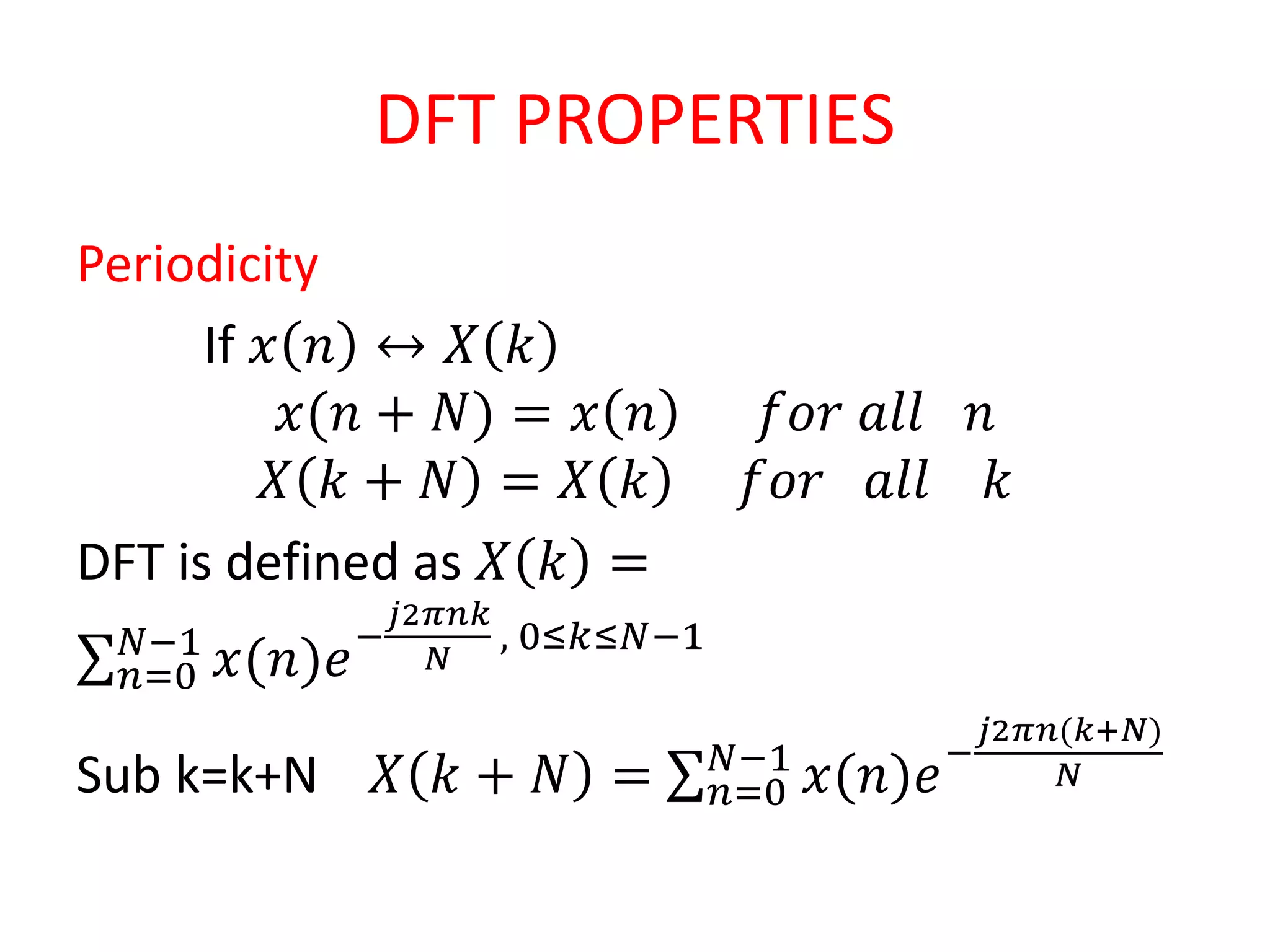
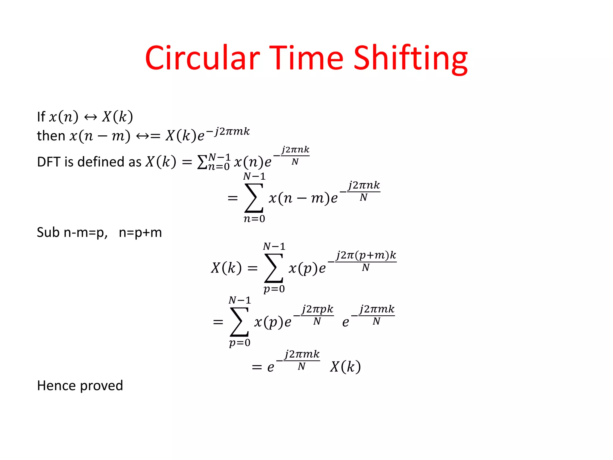
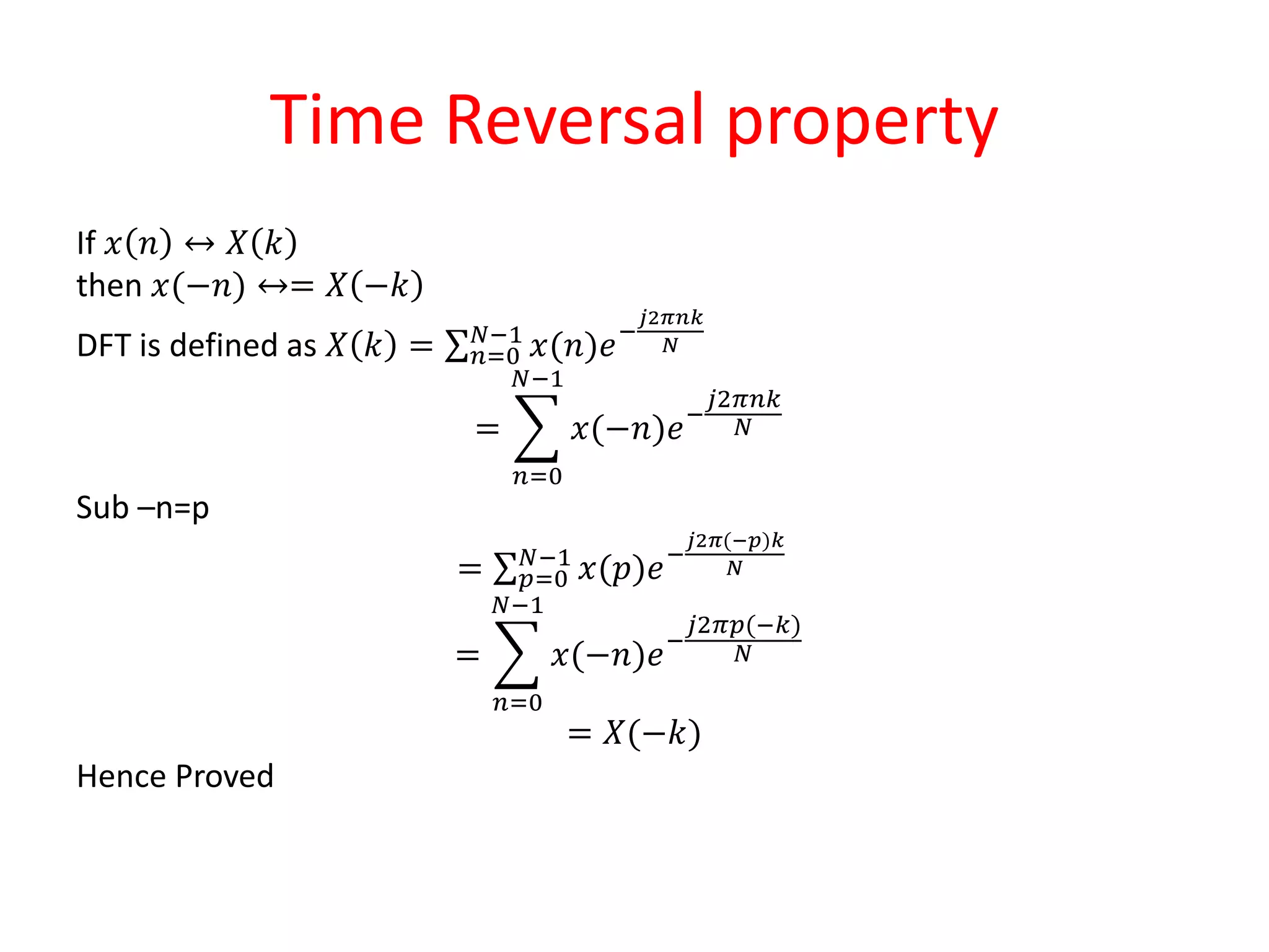
Transforms, such as the Fourier transform, make calculations involving signals easier by allowing analysis and computation to be done in either the time or frequency domain. The discrete Fourier transform (DFT) represents a signal as the sum of sinusoids at discrete frequencies. The DFT has several important properties including periodicity, linearity, time shifting, time reversal, and convolution. These properties allow signals to be analyzed and manipulated in the frequency domain.

1. Transforms
M.Starwin

2. Need for Transform
• Transforms make some types of calculations
much simpler and more convenient.
• Transforms are tools to make analysis easier.
• Laplace transform, for example, makes solving
differential equations easier.
• Possible to do all computation and analysis of
a signal in either the time domain or the
frequency domain.

3. Fourier Transform
















d
e
j
X
t
x
dt
e
t
x
j
X
t
j
t
j
)
(
2
1
)
(
)
(
)
(


4. Discrete Time Fourier Transform Pair









n
n
n
j
j
e
n
x
e
X )
(
)
(
Analysis


 





d
e
e
X
n
x n
j
j
)
(
2
1
)
(
Synthesis Inverse Fourier Transform
(IFT)
Fourier Transform
(FT)
)]
(
[
)
( n
x
e
X j
F


)]
(
[
)
( 1 
 j
-
e
X
n
x F
)
(
)
( 

 j
e
X
n
x F

5. Discrete Fourier Transform

6. DFT

7. IDFT

8. DFT PROPERTIES
Periodicity
If 𝑥 𝑛 ↔ 𝑋 𝑘
𝑥(𝑛 + 𝑁) = 𝑥 𝑛 𝑓𝑜𝑟 𝑎𝑙𝑙 𝑛
𝑋 𝑘 + 𝑁 = 𝑋 𝑘 𝑓𝑜𝑟 𝑎𝑙𝑙 𝑘
DFT is defined as 𝑋 𝑘 =
𝑛=0
𝑁−1
𝑥(𝑛)𝑒−
𝑗2𝜋𝑛𝑘
𝑁
, 0≤𝑘≤𝑁−1
Sub k=k+N 𝑋 𝑘 + 𝑁 = 𝑛=0
𝑁−1
𝑥(𝑛)𝑒−
𝑗2𝜋𝑛(𝑘+𝑁)
𝑁

9. Cond..
𝑋 𝑘 + 𝑁 =
𝑛=0
𝑁−1
𝑥(𝑛)𝑒−
𝑗2𝜋𝑛𝑘
𝑁 𝑒−
𝑗2𝜋𝑛𝑁
𝑁
𝑋 𝑘 + 𝑁 =
𝑛=0
𝑁−1
𝑥(𝑛)𝑒−
𝑗2𝜋𝑛𝑘
𝑁
[𝑒−𝑗2𝜋𝑛
= 1]
𝑋 𝑘 + 𝑁 = 𝑋 𝑘
Hence Proved.

10. Linearity
• If 𝑥1 𝑛 ↔ 𝑋1 𝑘 𝑎𝑛𝑑 𝑥2 𝑛 ↔ 𝑋2 𝑘
Then ∝ 𝑥1 𝑛 + β𝑥2 𝑛 ↔ α𝑋1 𝑘 + β𝑋2 𝑘
DFT is defined as 𝑋 𝑘 = 𝑛=0
𝑁−1
𝑥(𝑛)𝑒−
𝑗2𝜋𝑛𝑘
𝑁
=
𝑛=0
𝑁−1
[∝ 𝑥1 𝑛 + β𝑥2 𝑛 ]𝑒−
𝑗2𝜋𝑛𝑘
𝑁
=
𝑛=0
𝑁−1
∝ 𝑥1 𝑛 𝑒−
𝑗2𝜋𝑛𝑘
𝑁 +
𝑛=0
𝑁−1
β𝑥2 𝑛 𝑒−
𝑗2𝜋𝑛𝑘
𝑁
=∝
𝑛=0
𝑁−1
𝑥1 𝑛 𝑒−
𝑗2𝜋𝑛𝑘
𝑁 + β
𝑛=0
𝑁−1
𝑥2 𝑛 𝑒−
𝑗2𝜋𝑛𝑘
𝑁
=α𝑋1 𝑘 + β𝑋2 𝑘
Hence proved

11. Circular Time Shifting
If 𝑥 𝑛 ↔ 𝑋 𝑘
then 𝑥(𝑛 − 𝑚) ↔= 𝑋 𝑘 𝑒−𝑗2𝜋𝑚𝑘
DFT is defined as 𝑋 𝑘 = 𝑛=0
𝑁−1
𝑥(𝑛)𝑒−
𝑗2𝜋𝑛𝑘
𝑁
=
𝑛=0
𝑁−1
𝑥(𝑛 − 𝑚)𝑒−
𝑗2𝜋𝑛𝑘
𝑁
Sub n-m=p, n=p+m
𝑋 𝑘 =
𝑝=0
𝑁−1
𝑥(𝑝)𝑒−
𝑗2𝜋(𝑝+𝑚)𝑘
𝑁
=
𝑝=0
𝑁−1
𝑥(𝑝)𝑒−
𝑗2𝜋𝑝𝑘
𝑁 𝑒−
𝑗2𝜋𝑚𝑘
𝑁
= 𝑒−
𝑗2𝜋𝑚𝑘
𝑁 𝑋 𝑘
Hence proved

12. Time Reversal property
If 𝑥 𝑛 ↔ 𝑋 𝑘
then 𝑥(−𝑛) ↔= 𝑋 −𝑘
DFT is defined as 𝑋 𝑘 = 𝑛=0
𝑁−1
𝑥(𝑛)𝑒−
𝑗2𝜋𝑛𝑘
𝑁
=
𝑛=0
𝑁−1
𝑥(−𝑛)𝑒−
𝑗2𝜋𝑛𝑘
𝑁
Sub –n=p
= 𝑝=0
𝑁−1
𝑥(𝑝)𝑒−
𝑗2𝜋(−𝑝)𝑘
𝑁
=
𝑛=0
𝑁−1
𝑥(−𝑛)𝑒−
𝑗2𝜋𝑝(−𝑘)
𝑁
= 𝑋(−𝑘)
Hence Proved

13. Circular Convolution Property
If 𝑥1(𝑛) ↔ 𝑋𝑘 and 𝑥2 𝑛 ↔ 𝑋2 𝑘
then 𝑥1 𝑛 ∗ 𝑥2 𝑛 ↔ 𝑋1 𝑘 . 𝑋2 𝑘
DFT is defined as 𝑋 𝑘 = 𝑛=0
𝑁−1
𝑥(𝑛)𝑒−
𝑗2𝜋𝑛𝑘
𝑁
=
𝑛=0
𝑁−1
𝑥1 𝑛 ∗ 𝑥2 𝑛 ]𝑒−
𝑗2𝜋𝑛𝑘
𝑁
=
𝑛=0
𝑁−1
𝑚=0
𝑁−1
𝑥1 𝑚 𝑥2(𝑛 − 𝑚) 𝑒−
𝑗2𝜋𝑛𝑘
𝑁
[𝑥1 𝑛 ∗ 𝑥2 𝑛 = 𝑛=0
𝑁−1
𝑥1 𝑚 𝑥2 𝑛 − 𝑚 ]

14. Cond..
=
𝑚=0
𝑁−1
𝑥1(𝑚)
𝑛=0
𝑁−1
𝑥2(𝑛 − 𝑚) 𝑒−𝑗2𝜋𝑛𝑘/𝑁
= 𝑋2(k) 𝑚=0
𝑁−1
𝑥1(𝑚) 𝑒−𝑗2𝜋𝑚𝑘/𝑁
[using
time shift]
= 𝑋2 𝐾 𝑋1(𝐾)
Hence proved

15. Multiplication property
If 𝑥1(𝑛) ↔ 𝑋1(𝐾) and 𝑥2 𝑛 ↔ 𝑋2 𝑘
then 𝑥1 𝑛 𝑥2 𝑛 ↔ 1/𝑁[𝑋1 𝑘 ∗ 𝑋2 𝑘 ]
DFT is defined as 𝑋 𝑘 = 𝑛=0
𝑁−1
𝑥(𝑛)𝑒−
𝑗2𝜋𝑛𝑘
𝑁
=
𝑛=0
𝑁−1
𝑥1 𝑛 𝑥2 𝑛 𝑒−
𝑗2𝜋𝑛𝑘
𝑁
We know 𝑥1 𝑛 = 1/𝑁 𝑙=0
𝑁−1
𝑋1 𝑙 𝑒
𝑗2𝜋𝑛𝑙
𝑁
𝑋 𝑘 =
𝑛=0
𝑁−1
1/𝑁
𝑙=0
𝑁−1
𝑋1 𝑙 𝑒
𝑗2𝜋𝑛𝑙
𝑁 𝑥2 𝑛 𝑒−
𝑗2𝜋𝑛𝑘
𝑁

16. Cond..
=
1
𝑁
𝑙=0
𝑁−1
𝑋1(𝑙)
𝑛=0
𝑁−1
𝑥2(𝑛)𝑒−𝑗2𝜋𝑛(𝑘−𝑙)/𝑁
=
1
𝑁
𝑙=0
𝑁−1
𝑋1(𝑙)𝑋2(𝑘 − 𝑙)
=
1
𝑁
[𝑋1 𝑙 ∗ 𝑋2 𝑙 ]
=
1
𝑁
[𝑋1 𝑘 ∗ 𝑋2 𝑘 ]
Hence Proved.