Chapter-4 combined.pptx

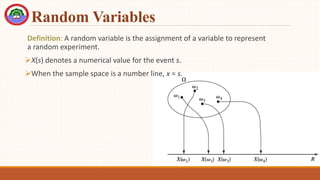
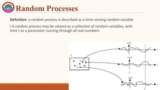
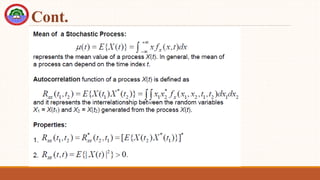
Introduction to Communication systems
(ECE- 3202)
Adama Science & Technology University
School of Electrical Engineering and Computing
Department of Electronics and Communication Engineering
Chapter 4
Review On Random And Stochastic Process

Review of Probability Theory
Probability theory is based on the phenomena that can be modeled by an
experiment with an outcome that is subject to chance.
Definition: A random experiment is repeated n time (n trials) and the
event A is observed m times (m occurrences). The probability is the
relative frequency of occurrence m/n.

Introduction to Probability and Random Variables
A deterministic signal can be derived by mathematical expressions.
A deterministic model (or system) will always produce the same output
from a given starting condition or initial state.
Stochastic (random) signals or processes፡
•Counterpart to a deterministic process
•Described in a probabilistic way
•Given initial condition, many realizations of the process exists

Cont.
Define the probability of an event A as:
𝑷 𝑨 =
𝑵𝑨
𝑵
where N is the number of possible
outcomes of the random experiment and
NA is the number of outcomes favorable to
the event A.
For example:
A 6-sided die has 6 outcomes.
3 of them are even,
Thus P(even) = 3/6

Axiomatic Definition of Probability
•A probability law (measure or function) that assigns probabilities to events
such that:
oP(A) ≥ 0
oP(S) =1
oIf A and B are disjoint events (mutually exclusive),
i.e. A ∩ B = ∅, then P(A ∪ B) = P(A) + P(B)
That is if A happens, B cannot occur.

Some Useful Properties
0 ≤ 𝑃(𝐴) ≤ 1
𝑃 ∅ = 0 : probability of impossible event
𝑃 𝐴 = 1 − 𝑃 𝐴 , 𝐴 the complement of A
If A and B are two events, then
𝑃 𝐴 ∪ 𝐵 = 𝑃 𝐴 + 𝑃 𝐵 − 𝑃 𝐴 ∩ 𝐵
If the sample space consits of n mutually exclusive events such that
𝑆 = 𝐴1 ∪ 𝐴2 ∪ ⋯ ∪ 𝐴𝑛, then
𝑃 𝑆 = 𝑃 𝐴1 + 𝑃 𝐴2 + ⋯ + 𝑃 𝐴𝑛 = 1

Joint and Marginal Probability
Joint probability:
is the likelihood of two events occurring together.
Joint probability is the probability of event A occurring at the same time
event B occurs.
It is P(A ∩ B) or P(AB).
Marginal probability:
is the probability of one event, ignoring any information about the other
event.
Thus P(A) and P(B) are marginal probabilities of events A and B

Conditional Probability
Let A and B be two events. The probability of event B given that event A
has occured is called the conditional probability.
𝑷 𝑨 𝑩 =
𝑷(𝑨∩𝑩)
𝑷(𝑩)
If the occurance of B has no effect on A, we say A and B are
indenpenderant events.
In this case 𝑷 𝑨 𝑩 = 𝑷(𝑨)
Combining both, we get 𝑷 𝑨 ∩ 𝑩 = 𝑷 𝑨 𝑷 𝑩 , when A and B are
indenpendent

Random Variables
Definition: A random variable is the assignment of a variable to represent
a random experiment.
X(s) denotes a numerical value for the event s.
When the sample space is a number line, x = s.

Cont.
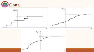
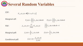
Definition: The cumulative distribution function (cdf) assigns a probability
value for the occurrence of x within a specified range such that FX(x) = P[X
≤ x].
Properties:
◦ 0 ≤ FX(x) ≤ 1
◦ FX(x1) ≤ FX(x2), if x1 ≤ x2
For discrete random variables FX(x) is a stair-case function.
Examples of CDFs for discrete, continuous, and mixed random variables
are shown

Cont.
Definition: The probability density function (pdf) is an alternative
description of the probability of the random variable X: fX(x) = d/dx FX(x)
P[x1 ≤ X ≤ x2] = P[X ≤ x2] - P[X ≤ x1]
= FX(x2) - FX(x1)
=  fX(x)dx over the interval [x1,x2]

Important Random Variables.
Bernoulli Random Variable. This is a discrete random variable taking two
values one and zero with probabilities p and 1 − p.
is a good model for a binary data generator.
a Bernoulli random variable can be employed to model the channel
errors.

Binomial Random Variable. This is a discrete random variable giving the
number of 1’s in a sequence of n independent Bernoulli trials.
The PMF is given by
This random variable models, for example,
the total number of bits received in error when
a sequence of n bits is transmitted over a
channel with bit-error probability of p.

Uniform Random Variable. This is a continuous random variable taking values
between a and b with equal probabilities over intervals of equal length.
The density function is given by
This is a model for continuous random variables whose range is known, but
nothing else is known about the likelihood of various values that the random
variable can assume.
For example, when the phase of a sinusoid is random it is usually modeled as a
uniform random variable between 0 and 2π.

Uniform Random Variable.

Gaussian or Normal Random Variable. This is a continuous random variable
described by the density function
The Gaussian random variable is the most important and frequently
encountered random variable in communications.
The reason is that thermal noise, which is the major source of noise in
communication systems, has a Gaussian distribution.

Gaussian or Normal Random Variable.

Several Random Variables
CDF:
Marginal cdf:
PDF:
Marginal pdf:
Conditional pdf:
 
y
Y
x
X
y
x
F Y
X 

 ,
)
,
(
, P
)
,
(
)
,
( ,
2
, y
x
F
y
x
y
x
f Y
X
Y
X



 1
)
,
(
, 
 






dv
du
v
u
f Y
X
 


 


x
Y
X
X dv
du
v
u
f
x
F )
,
(
)
( ,




 du
y
u
f
y
f Y
X
Y )
,
(
)
( ,




 dv
v
x
f
x
f Y
X
X )
,
(
)
( ,
 


 


y
Y
X
Y dv
du
v
u
f
y
F )
,
(
)
( ,
)
(
)
,
(
)
|
( ,
x
f
y
x
f
x
y
f
X
Y
X
Y 

Statistical Averages
The expected value of a random variable is a measure of the average of the value
that the random variable takes in a large number of experiments.
Function of a random variable:
   





 dx
x
xf
X X
X E

)
(X
g
Y 
     
     










 dx
x
f
X
g
X
g
dy
y
yf
Y X
Y E
E

Cont.
nth moments:
Central moments:
   




 dx
x
f
x
X X
n
n
E
   




 dx
x
f
x
X X
2
2
E
 
     






 dx
x
f
x
X X
n
X
n
X 

E
 
      2
2
2
X
X
X
X dx
x
f
x
X 

 


 



E
Mean-square value of X
Variance of X

Joint Moments
Correlation:
Covariance:
Correlation coefficient:
   
 






 dy
dx
y
x
f
y
x
Y
X Y
X
k
i
k
i
,
, ,
E Expected value of the product
- Also seen as a weighted inner product
   
   
 
 
  Y
X
XY
Y
Y
X
X
XY







E
E
E
E
cov
Correlation of the central moment
 






correlated
strongly
,
1
ed
uncorrelat
,
0
cov
Y
X
XY




Random Processes
Definition: a random process is described as a time-varying random variable
A random process may be viewed as a collection of random variables, with
time t as a parameter running through all real numbers.

Cont.
Mean of the random process:
Definition: a random process is first-order stationary if its pdf is constant
Definition: the autocorrelation is the expected value of the product of two
random variables at different times
   
    





 dx
x
xf
t
X
t t
X
X E

     
x
f
x
f t
X
t
X 2
1
   X
X t 
  Constant mean, variance
  2
2
X
X t 
 
     
 
2
1
2
1, t
X
t
X
t
t
RX E
    
2
1
2
1, t
t
R
t
t
R X
X 

Stationary to
second order

Cont.
Definition: the autocovariance of a stationary random process is
   
   
 
 
  2
2
1
2
1
2
1,
X
X
X
X
X
t
t
R
t
X
t
X
t
t
C








 E

Properties of Autocorrelation
Definition: autocorrelation of a stationary process only depends on the
time differences
Mean-square value:
Autocorrelation is an even function:
Autocorrelation has maximum at zero:
     
 
t
X
t
X
RX 
 
 E
   
 
t
X
RX
2
0 E

   

 
 X
X R
R
   
0
X
X R
R 


Example
Sinusoidal signal with random phase
Autocorrelation
   
 












otherwise
,
0
-
,
2
1
,
2
cos





t
f
t
f
A
t
X c
     
 
 





c
X
f
A
X
t
X
R
2
cos
2
2


 E As X(t) is compared to
itself at another time, we
see there is a periodic
behavior in correlation

Cross-correlation
Two random processes have the cross-correlation
Wide-sense stationary cross-correlation
   
     
 
u
Y
t
X
u
t
R
t
Y
t
X
XY E

,
,
       
   






XY
XY
Y
Y
X
X
R
u
R
u
R
u
R
t
R
t
R





,
,
,
,

Power Spectral Density
Definition: Fourier transform of autocorrelation function is called power spectral
density
Consider the units of X(t) Volts or Amperes
Autocorrelation is the projection of X(t) onto itself
Resulting units of Watts (normalized to 1 Ohm)
   
   











df
e
f
S
τ
R
dτ
e
R
f
S
f
j
X
X
f
j
X
X
2
2






Properties of PSD
Zero-frequency of PSD
Mean-square value
PSD is non-negative
PSD of a real-valued RP
   




 dτ
R
S X
X 0 
 
   




 df
f
S
t
X X
2
E
  0

f
SX
   
f
S
f
S X
X 


Example
Text Example
Mixing of a random process with a sinusoidal process
◦ Autocorrelation
◦ PSD
     


 t
f
t
X
t
Y c

2
cos
Wide-sense stationary RP
(to make it easier)
Uniformly distributed, but
not time-varying
     
     




 c
X
Y f
R
t
Y
t
Y
R 2
cos
2
1


 E
     
 
c
Y
c
Y
Y f
f
S
f
f
S
f
S 



4
1

Gaussian Process
The Gaussian probability density function for a single variable is
When the distribution has zero mean and unit variance
The random variable Y is said to be normally distributed as N(0,1)
   





 

 2
2
2
exp
2
1
Y
Y
Y
Y
y
y
f




  







2
exp
2
1 2
y
y
fY


Weakly Stationary
When we say that a process is stationary, we mean that it is weakly stationary, if
we do not explicitly say anything else.
A process that is not stationary is called non-stationary.
It is clear that every strictly stationary process with finite variance is also weakly
stationary.

Ensemble & Time Average
Mean and autocorrelation can be determined in two ways:
◦ The experiment can be repeated many times and the average taken over all these
functions. Such an average is called ensemble average.
◦ Take any one of these function as being representative of the ensemble and find
the average from a number of samples of this one function. This is called a time
average.
37

Ergodicity & Stationarity
If the time average and ensemble average of a random function are the same, it is
said to be ergodic.
A random function is said to be stationary if its statistics do not change as a
function of time.
◦ This is also called strict sense stationarity (vs. wide sense stationarity).
Any ergodic function is also stationary.
38

For a stationary signal we have:
Stationarity is defined as:
◦ Where
And the autocorrelation function is :
39
x
t
x 
)
(
)
,
,
(
)
,
,
,
( 2
1
2
1
2
1 
x
x
p
t
t
x
x
p 
1
2 t
t 




2
1,
2
1
2
1 )
,
,
(
)
(
x
x
x
x
p
x
x
r 


When x(t) is ergodic, its mean and autocorrelation are :
40






N
N
t
N
t
x
N
x )
(
2
1
lim
)
(
)
(
2
1
lim
)
(
)
(
)
( 

 








N
N
t
N
t
x
t
x
N
t
x
t
x
r

Cross-correlation
The cross-correlation of two ergodic random functions is :
◦ The subscript xy indicates a cross-correlation.
41









N
N
t
N
xy t
y
t
x
N
t
y
t
x
r )
(
)
(
1
lim
)
(
)
(
)
( 



Power & Cross Spectral Density
The Fourier transform of (the autocorrelation function of an ergodic
random function) is called the power spectral density of x(t) :
The cross-spectral density of two ergodic random functions is :
42









 j
e
r
S )
(
)
(









 j
xy
xy e
r
S )
(
)
(
)
(
r

Part -2
Review of types of Noise and calculation of Noise

Noise
 Noise is random signal that exists in communication systems
Noise in electrical terms may be defined as any unwanted introduction of energy tending to interfere
with the proper reception and reproduction of transmitted signals.

Cont.
• Practically, we cannot avoid the existence of unwanted signal together with the
modulated signal transmitted by the transmitter.
• This unwanted signal is called noise.
• Noise is random signal that exists in communication system.
• Random signal cannot be represented with a simple equation
• The existence of noise will degrade the level of quality of the received signal at
the receiver.

• Degrades system performance for both analog and digital system.
• The receiver cannot understand the sender
• The receiver cannot function as it should be.
• Reduce the efficiency of communication system.
Noise effect

1. External noise
External noise is defined as the type of Noise which is generated externally
External Noise are analyzed qualitatively.
Now, External Noise may be classified as
a) Atmospheric Noise : Atmospheric Noise is also known as static noise which is the
natural source of disturbance caused by lightning, discharge in thunderstorm and the
natural disturbances occurring in the nature.

b) Extraterrestrial Noise : Extraterrestrial Noise exist on the basis of their originating
source. They are subdivided into
i) Solar Noise
ii) Cosmic Noise
Solar noise is the noise that originates from the sun.
The sun radiates a broad spectrum of frequencies, including those, which are used for
broadcasting.
The sun is an active star and is constantly changing
Cont.

 Cosmic Noise
•Distant stars also radiate noise in much the same way as the sun.
•The noise received from them is called black body noise.
•Noise also comes from distant galaxies in much the same way as they come from the
milky way.
Cont.

c) Industrial Noise : Sources of Industrial noise are auto-mobiles, aircraft, ignition
of electric motors and switching gear.
The main cause of Industrial noise is High voltage wires. These noises is generally
produced by the discharge present in the operations.
Noise made by man easily outstrips any other between the frequencies of 1 to 600
MHz.
This includes such things as car and aircraft ignition, electric motors, switching equipment,
leakage from high voltage lines etc.
Cont.

 This is the noise generated by any of the active or passive devices found in the
receiver.
 This type of noise is random and difficult to treat on an individual basis but
can be described statistically.
 Random noise power is proportional to the bandwidth over which it is
measured.
2. Internal Noise

Types of internal noise
Internal Noise are the type of Noise which are generated internally or within the
Communication System or in the receiver.
Internal Noises are classified as
a) Shot Noise : These Noise are generally arises in the active devices due to the
random behavior of Charge particles or carries. In case of electron tube, shot
Noise is produces due to the random emission of electron form cathodes.
b) Partition Noise : When a circuit is to divide in between two or more paths then
the noise generated is known as Partition noise. The reason for the generation is
random fluctuation in the division.

Cont.
c) Low- Frequency Noise : They are also known as FLICKER NOISE. These type of
noise are generally observed at a frequency range below few kHz. Power spectral density
of these noise increases with the decrease in frequency. That why the name is given Low-
Frequency Noise.
d) High- Frequency Noise : These noises are also known TRANSIT- TIME Noise. They
are observed in the semi-conductor devices when the transit time of a charge carrier while
crossing a junction is compared with the time period of that signal.
e) Thermal Noise : Thermal Noise are random and often referred as White Noise or
Johnson Noise. Thermal noise are generally observed in the resistor or the sensitive
resistive components of a complex impedance due to the random and rapid movement of
molecules or atoms or electrons.

55
Cont.
 This type of noise is generated by all resistances
(e.g. a resistor, semiconductor, the resistance of a
resonant circuit, i.e. the real part of the impedance,
cable etc).
• electronic noise – generated by the thermal agitation of the charge carriers( the
electron) inside an electrical conductor in equilibrium, which happens regardless of
any applied voltage.
• Movement of electrons will form kinetic energy in the conductor related to the
temperature of the conductor.
• When the temperature increases, the movement of free electrons will increase and
the current flow through the conductor.
• Current flow due to the free electrons will create noise voltage, n(t).
• Noise voltage, n(t) is influenced by the temperature and therefore it is called thermal
noise.

Voltage and current models of a noisy resistor

Current model of noisy resistor

Addition of noise due to several sources in series

Addition of noise due to several sources in parallel

63
Resistance in Parallel
2
1
2
1
1
R
R
R
V
V n
o


2
1
1
2
2
R
R
R
V
V n
o


2
2
___
2
1
___
____
2
o
o
n V
V
V 


____
2
n
V
 
  









 2
1
2
1
2
2
2
1
1
1
2
2
2
2
1
4
R
R
R
R
R
T
R
R
T
R
R
R
kB
 2
2
1
2
2
1
1
2
1
_____
2 )
(
4
R
R
R
T
R
T
R
R
kB
Vn


 par
nr kTBR
R
R
R
R
kTB
V 4
4
2
1
2
1
_____
2











Proof:

Spectral densities of thermal noise

White noise
Noise in an idealized form is known as WHITE NOISE
WHITE NOISE contains all Frequency component in equal amount like white light consists
of all colors of light
If the probability of distribution of occurrence of a white noise is specified by a Gaussian
distribution function, then it is called White Gaussian noise.
Since power density spectrum of thermal and shot noise is independent of frequency, they
are referred as White Gaussian noise.
The power spectrum density of white noise is expressed as
Here the factor1/2 has been included to show that
half of the power is associated with the +ve frequencies
and remaining half with –ve frequencies shown in figure below.

Calculation of thermal noise for single noise source

Transfer function
   
 
 
 
 
     
 
 
  )
1
(
/
/
/
/
2
2
2
2
2
2
2
2
2










i
o
ni
i
no
o
ni
no
ni
no
ni
no
P
H
P
t
v
P
power
p
i
voltage
Noise
t
v
P
power
p
o
voltage
Noise
t
v
H
t
v
H
R
t
v
R
t
v
power
t
v
t
v
H




 
 
     
     








ni
no
ni
no
ni
i
no
o
S
H
S
BW
X
S
H
BW
X
S
eqn
from
BW
X
S
P
BW
X
S
P
BW
X
PSD
P
Power
2
2
)
1
(






Part-1
Part-2

Power relation with Power spectral density
PSD=POWER/BW
POWER=PSD X BW

Signal to noise ratio, noise figure, noise temperature,
calculation of noise figure.
Signal to noise ratio

Noise figure
Power gain, in decibels (dB), is defined as follows:
NOTE:

The noise factor of a device is related to its noise temperature Te
If several devices are cascaded, the total noise factor can be found with Friis' formula
where Fn is the noise factor for the n-th device, and Gn is the power gain (linear, not in dB) of the n-th
device.
The first amplifier in a chain usually has the most significant effect on the total noise figure because the
noise figures of the following stages are reduced by stage gains.
Noise Factor of a Device(Friis' formula)

Friis formula for noise factor
Friis's formula is used to calculate the total noise factor of a cascade of stages, each with its own noise
factor and power gain (assuming that the impedances are matched at each stage).
The total noise factor is given as
Friis's formula can be equivalently expressed in terms of noise temperature

Chapter-4 combined.pptx

More Related Content

Similar to Chapter-4 combined.pptx

Recently uploaded

Chapter-4 combined.pptx