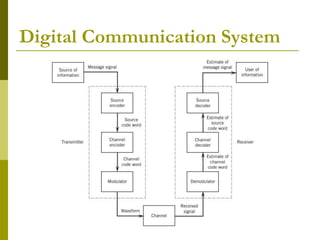
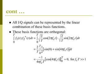
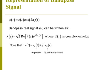
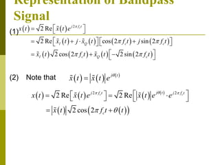
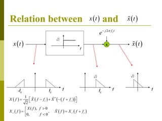
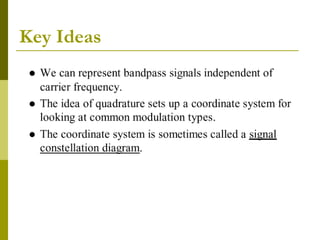
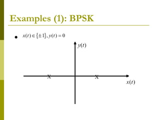
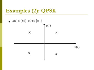
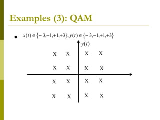
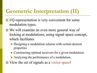
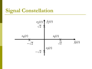
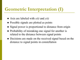
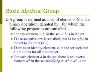
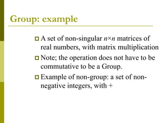
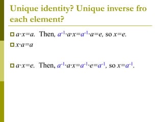
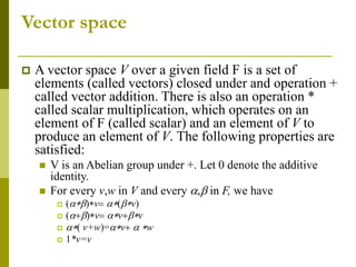
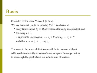
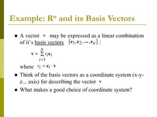
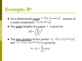
This document discusses signal-space analysis and representation of bandpass signals. It can be summarized as follows: 1) A bandpass real signal x(t) can be represented using its complex envelope x(t) and carrier frequency fc. This results in an in-phase (I) and quadrature-phase (Q) representation of the signal. 2) Signals can be viewed as vectors in a vector space. Basic algebra concepts like groups, fields, and vector spaces are introduced. 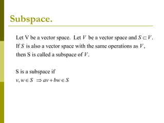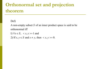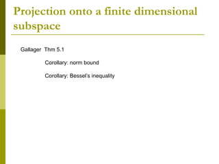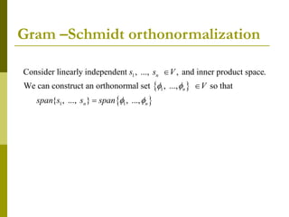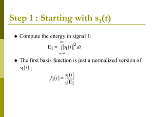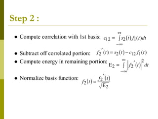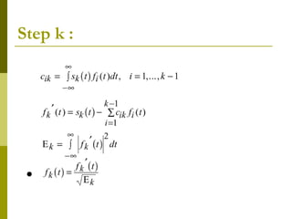3) Key concepts discussed include orthonormal bases, projection theorems, Gram-Schmidt orthonormalization, and representing signals in inner product spaces which allows defining notions of length and angle between signals.

1. Signal-Space Analysis
ENSC 428 – Spring 2008
Reference: Lecture 10 of Gallager

2. Digital Communication System

3. Representation of Bandpass
Signal
Bandpass real signal x(t) can be written as:
     
cos 2 c
x t s t f t


     
2
2 Re where is complex envelop
c
j f t
x t x t e x t

 
  
Note that      
I Q
x t x t j x t
  
In-phase Quadrature-phase

4. Representation of Bandpass
Signal
   
       
       
2
2 Re
2 Re cos 2 sin 2
2 cos 2 2 sin 2
c
j f t
I Q c c
I c Q c
x t x t e
x t j x t f t j f t
x t f t x t f t

 
 
 
  
 
   
 
 
 
 
  
 
(1)
(2) Note that      
j t
x t x t e


       
   
 
2 2
2 Re 2 Re
2 cos 2
c c
j t
j f t j f t
c
x t x t e x t e e
x t f t t

 
 
 
 
  
   
 

5. Relation between and
2
2
 
x t  
x t
f
x
2 c
j f t
e 

fc
-fc
f fc
f f
 
x t  
x t
     
 
     
*
1
2
( ), 0
,
0, 0
c c
c
X f X f f X f f
X f f
X f X f X f f
f
 
 
    
 


  



2

6. Energy of s(t)
 
 
 
 
2
2
2
0
2
0
(Rayleigh's energy theorem)
2 (Conjugate symmetry of real ( ) )
E s t dt
S f df
S f df s t
S f df















7. Representation of bandpass LTI
System
 
h t
 
h t
 
s t
 
s t
 
r t
 
r t
     
     
    because ( ) is band-limited.
c
r t s t h t
R f S f H f
S f H f f s t
 

 
     
 
 
   
*
( ), 0
0, 0
c c
c
H f H f f H f f
H f f
H f
f
H f H f f


 
    
 


 


 

8. Key Ideas

9. Examples (1): BPSK

10. Examples (2): QPSK

11. Examples (3): QAM

12. Geometric Interpretation (I)

13. Geometric Interpretation (II)
 I/Q representation is very convenient for some
modulation types.
 We will examine an even more general way of
looking at modulations, using signal space concept,
which facilitates
 Designing a modulation scheme with certain desired
properties
 Constructing optimal receivers for a given modulation
 Analyzing the performance of a modulation.
 View the set of signals as a vector space!

14. Basic Algebra: Group
 A group is defined as a set of elements G and a
binary operation, denoted by · for which the
following properties are satisfied
 For any element a, b, in the set, a·b is in the set.
 The associative law is satisfied; that is for a,b,c in
the set (a·b)·c= a·(b·c)
 There is an identity element, e, in the set such that
a·e= e·a=a for all a in the set.
 For each element a in the set, there is an inverse
element a-1 in the set satisfying a· a-1 = a-1 ·a=e.

15. Group: example
 A set of non-singular n×n matrices of
real numbers, with matrix multiplication
 Note; the operation does not have to be
commutative to be a Group.
 Example of non-group: a set of non-
negative integers, with +

16. Unique identity? Unique inverse fro
each element?
 a·x=a. Then, a-1·a·x=a-1·a=e, so x=e.
 x·a=a
 a·x=e. Then, a-1·a·x=a-1·e=a-1, so x=a-1.

17. Abelian group
 If the operation is commutative, the group is
an Abelian group.
 The set of m×n real matrices, with + .
 The set of integers, with + .

18. Application?
 Later in channel coding (for error correction or
error detection).

19. Algebra: field
 A field is a set of two or more elements
F={a,b,..} closed under two operations, +
(addition) and * (multiplication) with the
following properties
 F is an Abelian group under addition
 The set F−{0} is an Abelian group under
multiplication, where 0 denotes the identity
under addition.
 The distributive law is satisfied:
(a+bg  ag+bg

20. Immediately following properties
 ab0 implies a0 or b0
 For any non-zero a, a0 ?
 a0  a  a0  a 1 a0 1 a1a;
therefore a0 0
 00 ?
For a non-zero a, its additive inverse is non-zero.
00a a 0  a0 a0 000

21. Examples:
 the set of real numbers
 The set of complex numbers
 Later, finite fields (Galois fields) will be
studied for channel coding
 E.g., {0,1} with + (exclusive OR), * (AND)

22. Vector space
 A vector space V over a given field F is a set of
elements (called vectors) closed under and operation +
called vector addition. There is also an operation *
called scalar multiplication, which operates on an
element of F (called scalar) and an element of V to
produce an element of V. The following properties are
satisfied:
 V is an Abelian group under +. Let 0 denote the additive
identity.
 For every v,w in V and every a,b in F, we have
 (abv abv)
 (abv avbv
 a v+w)=av a w
 1*v=v

23. Examples of vector space
 Rn over R
 Cn over C
 L2 over

24. Subspace.
Let V be a vector space. Let be a vector space and .
If is also a vector space with the same operations as ,
then S is called a subspace of .
S is a subspace if
,
V S V
S V
V
v w S av bw S

   

25. Linear independence of vectors
1 2
Def)
A set of vectors , , are linearly independent iff
n
v v v V


26. Basis
0
Consider vector space V over F (a field).
We say that a set (finite or infinite) is a basis, if
* every finite subset of vectors of linearly independent, and
* for every ,
it
B V
B B
x V



1 1
1 1
is possible to choose , ..., and , ...,
such that ... .
The sums in the above definition are all finite because without
additional structure the axioms of a vector
n n
n n
a a F v v B
x a v a v
 
  
space do not permit us
to meaningfully speak about an infinite sum of vectors.

27. Finite dimensional vector space
1 2
1 2
A set of vectors , , is said to span if
every vector is a linear combination of , , .
Example:
n
n
n
v v v V V
u V v v v
R



28. Finite dimensional vector space
 A vector space V is finite dimensional if there
is a finite set of vectors u1, u2, …, un that span V.

29. Finite dimensional vector space
1 2
1 2
1 2
Let V be a finite dimensional vector space. Then
If , , are linearly independent but do not span , then
has a basis with vectors ( ) that include , , .
If , , span and but ar
m
m
m
v v v V V
n n m v v v
v v v V



1 2
e linearly dependent, then
a subset of , , is a basis for with vectors ( ) .
Every basis of contains the same number of vectors.
Dimension of a finiate dimensional vector space.
m
v v v V n n m
V



30. Example: Rn and its Basis Vectors




31. Inner product space: for length and
angle

32. Example: Rn













33. Orthonormal set and projection
theorem
Def)
A non-empty subset of an inner product space is said to be
orthonormal iff
1) , , 1 and
2) If , and , then , 0.
S
x S x x
x y S x y x y
   
   

34. Projection onto a finite dimensional
subspace
Gallager Thm 5.1
Corollary: norm bound
Corollary: Bessel’s inequality

35. Gram –Schmidt orthonormalization
 
 
1
1
1 1
Consider linearly independent , ..., , and inner product space.
We can construct an orthonormal set , ..., so that
{ , ..., } , ...,
n
n
n n
s s V
V
span s s span
 
 




36. Gram-Schmidt Orthog. Procedure

37. Step 1 : Starting with s1(t)

38. Step 2 :

39. Step k :

40. Key Facts

41. Examples (1)

42. cont … (step 1)

43. cont … (step 2)

44. cont … (step 3)

45. cont … (step 4)

46. Example application of projection
theorem
Linear estimation

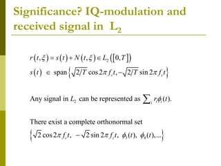
47. L2([0,T])
(is an inner product space.)
 
 
 
2
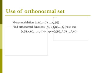
Consider an orthonormal set
1 2
exp 0, 1, 2,... .
Any function ( ) in 0, is , . Fourier series.
For this reason, this orthonormal set is called complete
k
k k
k
kt
t j k
T
T
u t L T u u


 


 
 
   
 
 
 
 
 
2
.
Thm: Every orthonormal set in is contained in some
complete orthonormal set.
Note that the complete orthonormal set above is not unique.
L

48. Significance? IQ-modulation and
received signal in L2
       
 
   
 
2
2
3 4
, , 0,
span 2 cos2 , 2 sin 2
Any signal in can be represented as ( ).
There exist a complete orthonormal set
2 cos2 , 2 sin 2 , ( ), ( ),...
c c
i i
i
c c
r t s t N t L T
s t T f t T f t
L r t
f t f t t t
 
 

   
  
 



49. On Hilbert space over C. For special
folks (e.g., mathematicians) only
L2 is a separable Hilbert space. We have very useful
results on
1) isomorphism 2)countable complete orthonormal set
Thm
If H is separable and infinite dimensional, then it is
isomorphic to l2 (the set of square summable sequence
of complex numbers)
If H is n-dimensional, then it is isomorphic to Cn.
The same story with Hilbert space over R. In some sense there is only one real and one
complex infinite dimensional separable Hilbert space.
L. Debnath and P. Mikusinski, Hilbert Spaces with Applications, 3rd Ed., Elsevier, 2005.

50. Hilbert space
Def)
A complete inner product space.
Def) A space is complete if every Cauchy
sequence converges to a point in the space.
Example: L2

51. Orthonormal set S in Hilbert space
H is complete if
2
2
Equivalent definitions
1) There is no other orthonormal set strictly containing . (maximal)
2) , ,
3) , , implies 0
4) , ,
Here, we do not need to assume H is separable.
i i
i
S
x H x x e e
x e e S x
x H x x e
  
  
  


Summations in 2) and 4) make sense because we can prove the following:

52. Only for mathematicians (We don’t
need separability.)
 
 
2 2
Let be an orthonormal set in a Hilbert space .
For each vector x , set , 0 is
either empty or countable.
Proof: Let , .
Then, (finite)
Also, any element in (however small
n
n
O H
H S e O x e
S e O x e x n
S n
e S
   
  

1
, is)
is in for some (sufficiently large).
Therefore, . Countable.
n
n
n
x e
S n
S S




53. Theorem
 Every orothonormal set in a Hilbert space is
contained in some complete orthonormal set.
 Every non-zero Hilbert space contains a complete
orthonormal set.
 (Trivially follows from the above.)
( “non-zero” Hilbert space means that the space has a non-zero element.
We do not have to assume separable Hilbert space.)
 Reference: D. Somasundaram, A first course in functional analysis, Oxford, U.K.: Alpha Science, 2006.

54. Only for mathematicians.
(Separability is nice.)
Euivalent definitions
Def) is separable iff there exists a countable subset
which is dense in , that is, .
Def) is separable iff there exists a countable subset such that
,
H D
H D H
H D
x H

  there exists a sequence in convergeing to .
Thm: If has a countable complete orthonormal set, then is separable.
proof: set of linear combinations (loosely speaking)
D x
H H
with ratioanl real and imaginary parts. This set is dense (show sequence)
Thm: If is separable, then every orthogonal set is countable.
proof: normalize it. Distance between two orthonorma
H
l elements is 2. .....

55. Signal Spaces:
L2 of complex functions

56. Use of orthonormal set
1 2
1 2
1 2 1 2
M-ary modulation { ( ), ( ),..., ( )}
Find orthonormal functions ( ), ( ),.., ( ) so that
{ ( ), ( ),..., ( )} { ( ), ( ),.., ( )}
M
K
M K
s t s t s t
f t f t f t
s t s t s t span f t f t f t


57. Examples (1)
2
T
2
T

58. Signal Constellation

59. cont …

60. cont …

61. cont …
QPSK

62. Examples (2)

63. Example: Use of orthonormal set
and basis
 Two square functions

64. Signal Constellation

65. Geometric Interpretation (III)

66. Key Observations

67. Vector XTMR/RCVR Model
 
 
 

  
1 t   
1 t
  
 t   
 t
r = s + n
1 1 1
s1
Vector
RCVR
Vector
XTMR
Waveform channel / Correlation
Receiver
s(t)
n(t)
r(t)
s2
sN
r = s + n
2 2 2
r = s + n
N N N
  
 t   
 t


s(t)
n(t)
r(t) = s(t) + n(t)
0
T
z
0
T
z
0
T
z
}
i 1



i 1
N

   ,  
i i j
t i = j
 
i t
si
ni
s(t) =
n(t) =
A
.
.
.
.
.
.
.
.
.
.
.
.