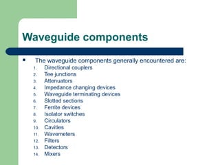
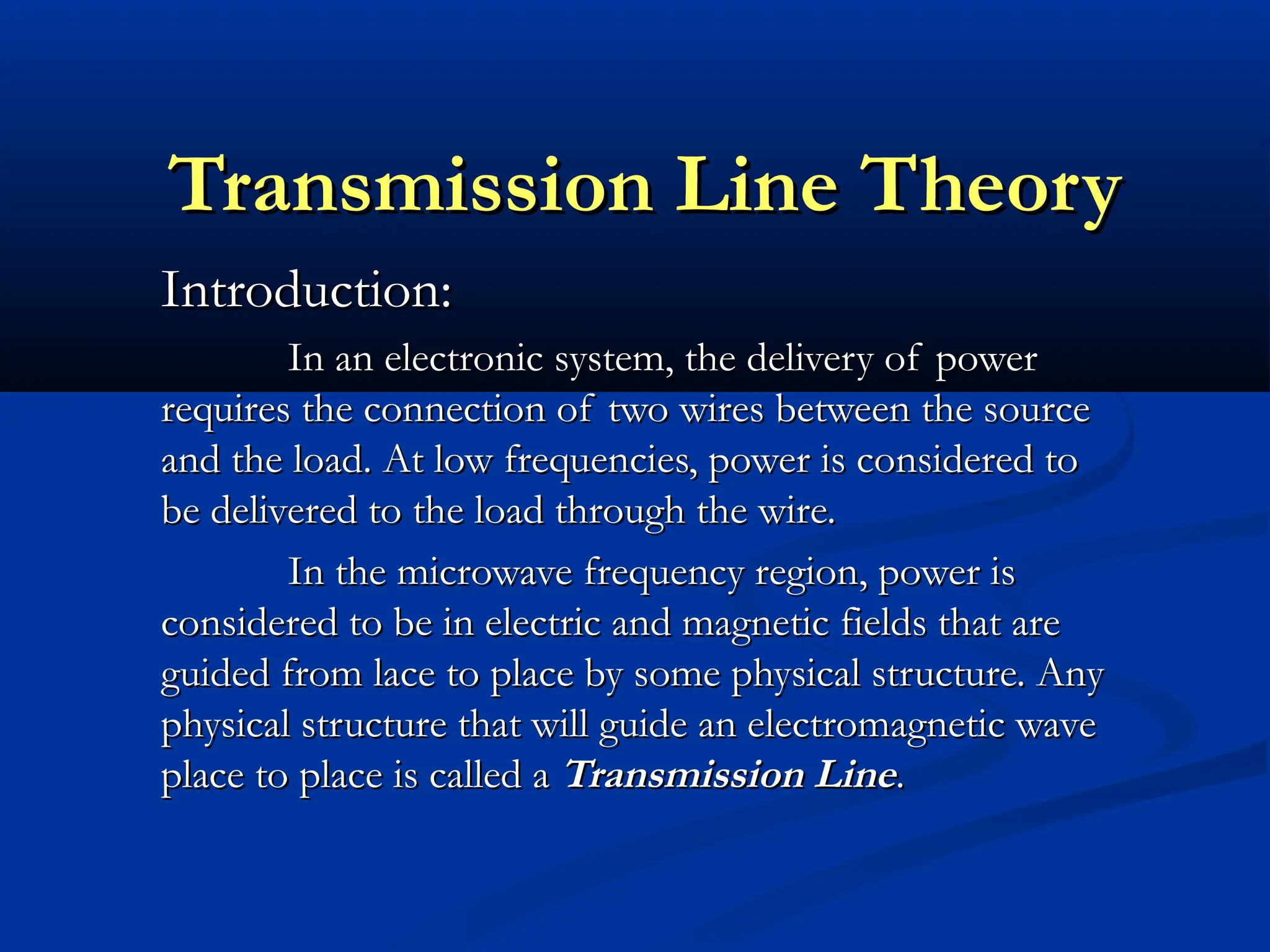
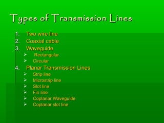
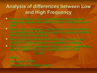
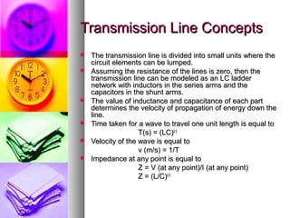
SlideShare a Scribd company logo
Transmission Line Theory
Introduction:
Introduction:
In an electronic system, the delivery of power
requires the connection of two wires between the source
and the load. At low frequencies, power is considered to
be delivered to the load through the wire.
In the microwave frequency region, power is
considered to be in electric and magnetic fields that are
guided from lace to place by some physical structure. Any
physical structure that will guide an electromagnetic wave
place to place is called a
place to place is called a Transmission Line
Transmission Line.
.
Types of Transmission Lines
1.
1. Two wire line
Two wire line
2.
2. Coaxial cable
Coaxial cable
3.
3. Waveguide
Waveguide
 Rectangular
Rectangular
 Circular
Circular
4.
4. Planar Transmission Lines
Planar Transmission Lines
 Strip line
Strip line
 Microstrip line
Microstrip line
 Slot line
Slot line
 Fin line
Fin line
 Coplanar Waveguide
Coplanar Waveguide
 Coplanar slot line
Coplanar slot line
Analysis of differences between Low
and High Frequency
and High Frequency
 At low frequencies, the circuit elements are lumped since
At low frequencies, the circuit elements are lumped since
voltage and current waves affect the entire circuit at the same
time.
time.
 At microwave frequencies, such treatment of circuit elements
At microwave frequencies, such treatment of circuit elements
is not possible since voltag and current waves do not affect the
entire circuit at the same time.
 The circuit must be broken down into unit sections within
The circuit must be broken down into unit sections within
which the circuit elements are considered to be lumped.
 This is because the dimensions of the circuit are comparable to
This is because the dimensions of the circuit are comparable to
the wavelength of the waves according to the formula:

c/f
c/f
where,
where,
c = velocity of light
f = frequency of voltage/current
Transmission Line Concepts
 The transmission line is divided into small units where the
The transmission line is divided into small units where the
circuit elements can be lumped.
 Assuming the resistance of the lines is zero, then the
Assuming the resistance of the lines is zero, then the
transmission line can be modeled as an LC ladder
network with inductors in the series arms and the
capacitors in the shunt arms.
 The value of inductance and capacitance of each part
The value of inductance and capacitance of each part
determines the velocity of propagation of energy down the
line.
line.
 Time taken for a wave to travel one unit length is equal to
Time taken for a wave to travel one unit length is equal to
T(s) = (LC)
T(s) = (LC)0.5
0.5
 Velocity of the wave is equal to
Velocity of the wave is equal to
v (m/s) = 1/T
v (m/s) = 1/T
 Impedance at any point is equal to
Impedance at any point is equal to
Z = V (at any point)/I (at any point)
Z = (L/C)
Z = (L/C)0.5
0.5
Line terminated in its characteristic
impedance: If the end of the transmission line is
terminated in a resistor equal in value to the
characteristic impedance of the line as calculated
by the formula Z=(L/C)0.5
, then the voltage and
current are compatible and no reflections occur.
Line terminated in a short: When the end of the
transmission line is terminated in a short (RL= 0),
the voltage at the short must be equal to the
product of the current and the resistance.
Line terminated in an open: When the line is
terminated in an open, the resistance between the
open ends of the line must be infinite. Thus the
current at the open end is zero.
Reflection from Resistive loads
► When the resistive load termination is not equal to the
When the resistive load termination is not equal to the
characteristic impedance, part of the power is reflected
back and the remainder is absorbed by the load. The
amount of voltage reflected back is called
amount of voltage reflected back is called voltage reflection
voltage reflection
coefficient.
coefficient.

V
Vr
r/V
/Vii
where V
where Vr
r = incident voltage
= incident voltage
V
Vii = reflected voltage
= reflected voltage
► The reflection coefficient is also given by
The reflection coefficient is also given by

 = (Z
= (ZL
L - Z
- ZO
O)/(Z
)/(ZL
L + Z
+ ZO
O)
)
Standing Waves
Standing Waves
 A standing wave is formed by the addition of incident and reflected waves
A standing wave is formed by the addition of incident and reflected waves
and has nodal points that remain stationary with time.
 Voltage Standing Wave Ratio:
Voltage Standing Wave Ratio:
VSWR = V
VSWR = Vmax
max/V
/Vmin
min
 Voltage standing wave ratio expressed in decibels is called the
Voltage standing wave ratio expressed in decibels is called the Standing
Standing
Wave Ratio:
Wave Ratio:
SWR (dB) = 20log
SWR (dB) = 20log10
10VSWR
VSWR
 The maximum impedance of the line is given by:
The maximum impedance of the line is given by:
Z
Zmax
max = V
= Vmax
max/I
/Imin
min
 The minimum impedance of the line is given by:
The minimum impedance of the line is given by:
Z
Zmin
min = V
= Vmin
min/I
/Imax
max
or alternatively:
or alternatively:
Z
Zmin
min = Z
= Zo
o/VSWR
/VSWR
 Relationship between VSWR and Reflection Coefficient:
Relationship between VSWR and Reflection Coefficient:
VSWR = (1 +
VSWR = (1 + 
1 -
1 - 


(VSWR – 1)/(VSWR + 1)
(VSWR – 1)/(VSWR + 1)
General Input Impedance Equation
 Input impedance of a transmission line at a
distance L from the load impedance ZLwith a
characteristic Zo is
Zinput = Zo [(ZL + j Zo BL)/(Zo + j ZL BL)]
where B is called phase constant or
wavelength constant and is defined by the
equation
B = 2
Half and Quarter wave transmission lines
 The relationship of the input impedance at the
The relationship of the input impedance at the
input of the half-wave transmission line with its
terminating impedance is got by letting L =

in the impedance equation.
in the impedance equation.
Z
Zinput
input = Z
= ZL
L 

 The relationship of the input impedance at the
The relationship of the input impedance at the
input of the quarter-wave transmission line with
its terminating impedance is got by letting L =

in the impedance equation.
in the impedance equation.
Z
Zinput
input = (Z
= (Zinput
input Z
Zoutput
output)
)0.5
0.5


Effect of Lossy line on voltage and
current waves
current waves
 The effect of resistance in a transmission line is to continuously
The effect of resistance in a transmission line is to continuously
reduce the amplitude of both incident and reflected voltage and
current waves.
current waves.
 Skin Effect:
Skin Effect: As frequency increases, depth of penetration into
As frequency increases, depth of penetration into
adjacent conductive surfaces decreases for boundary currents
associated with electromagnetic waves. This results in the
confinement of the voltage and current waves at the boundary of
the transmission line, thus making the transmission more lossy.
 The skin depth is given by:
The skin depth is given by:
skin depth (m) = 1
skin depth (m) = 1
f
f
0.5
0.5
where f = frequency, Hz

= permeability, H/m
= permeability, H/m

= conductivity, S/m
= conductivity, S/m

Smith chart
Smith chart
► For complex transmission line problems, the use
For complex transmission line problems, the use
of the formulae becomes increasingly difficult and
inconvenient. An indispensable graphical method
of solution is the use of Smith Chart.
Components of a Smith Chart
 Horizontal line:
Horizontal line: The horizontal line running through the
The horizontal line running through the
center of the Smith chart represents either the resistive ir the
conductive component. Zero resistance or conductance is
located on the left end and infinite resistance or conductance is
located on the right end of the line.
 Circles of constant resistance and conductance:
Circles of constant resistance and conductance: Circles of
Circles of
constant resistance are drawn on the Smith chart tangent to the
right-hand side of the chart and its intersection with the
centerline. These circles of constant resistance are used to
locate complex impedances and to assist in obtaining solutions
to problems involving the Smith chart.
 Lines of constant reactance:
Lines of constant reactance: Lines of constant reactance are
Lines of constant reactance are
shown on the Smith chart with curves that start from a given
reactance value on the outer circle and end at the right-hand
side of the center line.
Solutions to Microwave problems using Smith chart
 The types of problems for which Smith charts are used
include the following:
1. Plotting a complex impedance on a Smith chart
2. Finding VSWR for a given load
3. Finding the admittance for a given impedance
4. Finding the input impedance of a transmission line terminated
in a short or open.
5. Finding the input impedance at any distance from a load ZL.
6. Locating the first maximum and minimum from any load
7. Matching a transmission line to a load with a single series
stub.
8. Matching a transmission line with a single parallel stub
9. Matching a transmission line to a load with two parallel stubs.
Plotting a Complex Impedance on a Smith Chart
 To locate a complex impedance, Z = R+-jX or
admittance Y = G +- jB on a Smith chart,
normalize the real and imaginary part of the
complex impedance. Locating the value of the
normalized real term on the horizontal line scale
locates the resistance circle. Locating the
normalized value of the imaginary term on the
outer circle locates the curve of constant
reactance. The intersection of the circle and the
curve locates the complex impedance on the
Smith chart.
Finding the VSWR for a given load
Normalize the load and plot its location on
the Smith chart.
Draw a circle with a radius equal to the
distance between the 1.0 point and the
location of the normalized load and the
center of the Smith chart as the center.
The intersection of the right-hand side of
the circle with the horizontal resistance
line locates the value of the VSWR.
Finding the Input Impedance at any
Distance from the Load
 The load impedance is first normalized and is
located on the Smith chart.
 The VSWR circle is drawn for the load.
 A line is drawn from the 1.0 point through the
load to the outer wavelength scale.
 To locate the input impedance on a Smith chart
of the transmission line at any given distance
from the load, advance in clockwise direction
from the located point, a distance in wavelength
equal to the distance to the new location on the
transmission line.
Power Loss
 Return Power Loss: When an electromagnetic wave
travels down a transmission line and encounters a
mismatched load or a discontinuity in the line, part of the
incident power is reflected back down the line. The return
loss is defined as:
Preturn = 10 log10 Pi/Pr
Preturn = 20 log10 1/
 Mismatch Power Loss: The term mismatch loss is used
to describe the loss caused by the reflection due to a
mismatched line. It is defined as
Pmismatch = 10 log10 Pi/(Pi - Pr)
Microwave Components
 Microwave components do the following functions:
1. Terminate the wave
2. Split the wave into paths
3. Control the direction of the wave
4. Switch power
5. Reduce power
6. Sample fixed amounts of power
7. Transmit or absorb fixed frequencies
8. Transmit power in one direction
9. Shift the phase of the wave
10. Detect and mix waves
Coaxial components
 Connectors: Microwave coaxial connectors required to connect two
coaxial lines are als called connector pairs (male and female). They
must match the characteristic impedance of the attached lines and be
designed to have minimum reflection coefficients and not radiate
power through the connector.
E.g. APC-3.5, BNC, SMA, SMC, Type N
 Coaxial sections: Coaxial line sections slip inside each other while
still making electrical contact. These sections are useful for matching
loads and making slotted line measurements. Double and triple stub
tuning configurations are available as coaxial stub tuning sections.
 Attenuators: The function of an attenuator is to reduce the power of
the signal through it by a fixed or adjustable amount. The different
types of attenuators are:
1. Fixed attenuators
2. Step attenuators
3. Variable attenuators
Coaxial components (contd.)
 Coaxial cavities: Coaxial cavities are
concentric lines or coaxial lines with an air
dielectric and closed ends. Propagation of
EM waves is in TEM mode.
 Coaxial wave meters: Wave meters use a
cavity to allow the transmission or absorption
of a wave at a frequency equal to the
resonant frequency of the cavity. Coaxial
cavities are used as wave meters.
Waveguide components
 The waveguide components generally encountered are:
1. Directional couplers
2. Tee junctions
3. Attenuators
4. Impedance changing devices
5. Waveguide terminating devices
6. Slotted sections
7. Ferrite devices
8. Isolator switches
9. Circulators
10. Cavities
11. Wavemeters
12. Filters
13. Detectors
14. Mixers
Tees
 Hybrid Tee junction: Tee junctions are used
to split waves from one waveguide to two
other waveguides. There are two ways of
connecting the third arm to the waveguide –
1. along the long dimension, called E=plane Tee.
2. along the narrow dimension, called H-Plane Tee
 Hybrid Tee junction: the E-plane and H-
plane tees can be combined to form a
hybrid tee junction called Magic Tee
Attenuators
 Attenuators are components that reduce the amount of power a fixed
amount, a variable amount or in a series of fixed steps from the input
to the output of the device. They operate on the principle of interfering
with the electric field or magnetic field or both.
 Slide vane attenuators: They work on the principle that a resistive
material placed in parallel with the E-lines of a field current will induce
a current in the material that will result in I2
R power loss.
 Flap attenuator: A flap attenuator has a vane that is dropped into the
waveguide through a slot in the top of the guide. The further the vane
is inserted into the waveguide, the greater the attenuation.
 Rotary vane attenuator: It is a precision waveguide attenuator in which
attenuation follows a mathematical law. In this device, attenuation is
independent on frequency.
Isolators
 Mismatch or discontinuities cause energy to be reflected back
down the line. Reflected energy is undesirable. Thus, to
prevent reflected energy from reaching the source, isolators are
used.
 Faraday Rotational Isolator: It combines ferrite material to
shift the phase of an electromagnetic wave in its vicinity and
attenuation vanes to attenuate an electric field that is parallel to
the resistive plane.
 Resonant absorption isolator: A device that can be used for
higher powers. It consists of a section of rectangular waveguide
with ferrite material placed half way to the center of the
waveguide, along the axis of the guide.

More Related Content

Similar to 519transmissionlinetheory-130315033930-phpapp02.pdf

BASIC CONCEPTS OF TRANSMISSION LINES & WAVEGUIDES ForC 18 DECE unit 1, SBTET
BASIC CONCEPTS OF TRANSMISSION LINES  &  WAVEGUIDES ForC 18 DECE unit 1, SBTETBASIC CONCEPTS OF TRANSMISSION LINES  &  WAVEGUIDES ForC 18 DECE unit 1, SBTET
BASIC CONCEPTS OF TRANSMISSION LINES & WAVEGUIDES ForC 18 DECE unit 1, SBTET
janakiravi
 
chapter 3 part 1.ppt
chapter 3 part 1.pptchapter 3 part 1.ppt
chapter 3 part 1.ppt
ErmiyasSolomon2
 
Transmission lines and waveguides -Two marks
Transmission lines and waveguides -Two marksTransmission lines and waveguides -Two marks
Transmission lines and waveguides -Two marks
Dr.SHANTHI K.G
 
EC8651 Transmissions lines and RF systems-two marks
EC8651  Transmissions lines and RF systems-two marksEC8651  Transmissions lines and RF systems-two marks
EC8651 Transmissions lines and RF systems-two marks
Dr.SHANTHI K.G
 
TLW_Unit I material pdf.ppt
TLW_Unit I material pdf.pptTLW_Unit I material pdf.ppt
TLW_Unit I material pdf.ppt
KanmaniRajamanickam
 
Transmission lines
Transmission linesTransmission lines
Transmission lines
Suneel Varma
 
lecture note AC fundamental LESSON 2.pptx
lecture note AC fundamental LESSON 2.pptxlecture note AC fundamental LESSON 2.pptx
lecture note AC fundamental LESSON 2.pptx
kifle203
 
transmission line
 transmission line transmission line
transmission line
MONEERTHAMEER
 
transmission line theory prp
transmission line theory prptransmission line theory prp
transmission line theory prp
Dr. Pravin Prajapati
 
2 Port Networks
2 Port Networks2 Port Networks
2 Port Networks
Manjunath Achari
 
Cp13.pptx
Cp13.pptxCp13.pptx
Cp13.pptx
DOAFCLF
 
AC FUNDAMENTALS.pptx
AC FUNDAMENTALS.pptxAC FUNDAMENTALS.pptx
AC FUNDAMENTALS.pptx
roshan375533
 
halfwave antenaa dipole antenna qurter wave.pptx
halfwave antenaa dipole antenna qurter wave.pptxhalfwave antenaa dipole antenna qurter wave.pptx
halfwave antenaa dipole antenna qurter wave.pptx
mshanajoel6
 
Electrical transmission line
Electrical transmission lineElectrical transmission line
Electrical transmission line
Dhananjay Jha
 
Series parallel resonance circuit
Series parallel resonance circuitSeries parallel resonance circuit
Series parallel resonance circuit
Praveen Vaidya
 
lattice diagram.ppt
lattice diagram.pptlattice diagram.ppt
lattice diagram.ppt
krishnakumars92
 
01 Lecture Transmission Lines 01.pptx
01 Lecture Transmission Lines 01.pptx01 Lecture Transmission Lines 01.pptx
01 Lecture Transmission Lines 01.pptx
BashirAhmed396449
 
Ap unit 1
Ap unit 1Ap unit 1
Ap unit 1
vinutnaujwalag
 
CT UNIT-III.pptx
CT UNIT-III.pptxCT UNIT-III.pptx
CT UNIT-III.pptx
sasitharjaisankaran1
 
Single phase AC circuits
Single phase AC circuitsSingle phase AC circuits
Single phase AC circuits
Pranav Gupta
 

Similar to 519transmissionlinetheory-130315033930-phpapp02.pdf (20)

BASIC CONCEPTS OF TRANSMISSION LINES & WAVEGUIDES ForC 18 DECE unit 1, SBTET
BASIC CONCEPTS OF TRANSMISSION LINES  &  WAVEGUIDES ForC 18 DECE unit 1, SBTETBASIC CONCEPTS OF TRANSMISSION LINES  &  WAVEGUIDES ForC 18 DECE unit 1, SBTET
BASIC CONCEPTS OF TRANSMISSION LINES & WAVEGUIDES ForC 18 DECE unit 1, SBTET
 
chapter 3 part 1.ppt
chapter 3 part 1.pptchapter 3 part 1.ppt
chapter 3 part 1.ppt
 
Transmission lines and waveguides -Two marks
Transmission lines and waveguides -Two marksTransmission lines and waveguides -Two marks
Transmission lines and waveguides -Two marks
 
EC8651 Transmissions lines and RF systems-two marks
EC8651  Transmissions lines and RF systems-two marksEC8651  Transmissions lines and RF systems-two marks
EC8651 Transmissions lines and RF systems-two marks
 
TLW_Unit I material pdf.ppt
TLW_Unit I material pdf.pptTLW_Unit I material pdf.ppt
TLW_Unit I material pdf.ppt
 
Transmission lines
Transmission linesTransmission lines
Transmission lines
 
lecture note AC fundamental LESSON 2.pptx
lecture note AC fundamental LESSON 2.pptxlecture note AC fundamental LESSON 2.pptx
lecture note AC fundamental LESSON 2.pptx
 
transmission line
 transmission line transmission line
transmission line
 
transmission line theory prp
transmission line theory prptransmission line theory prp
transmission line theory prp
 
2 Port Networks
2 Port Networks2 Port Networks
2 Port Networks
 
Cp13.pptx
Cp13.pptxCp13.pptx
Cp13.pptx
 
AC FUNDAMENTALS.pptx
AC FUNDAMENTALS.pptxAC FUNDAMENTALS.pptx
AC FUNDAMENTALS.pptx
 
halfwave antenaa dipole antenna qurter wave.pptx
halfwave antenaa dipole antenna qurter wave.pptxhalfwave antenaa dipole antenna qurter wave.pptx
halfwave antenaa dipole antenna qurter wave.pptx
 
Electrical transmission line
Electrical transmission lineElectrical transmission line
Electrical transmission line
 
Series parallel resonance circuit
Series parallel resonance circuitSeries parallel resonance circuit
Series parallel resonance circuit
 
lattice diagram.ppt
lattice diagram.pptlattice diagram.ppt
lattice diagram.ppt
 
01 Lecture Transmission Lines 01.pptx
01 Lecture Transmission Lines 01.pptx01 Lecture Transmission Lines 01.pptx
01 Lecture Transmission Lines 01.pptx
 
Ap unit 1
Ap unit 1Ap unit 1
Ap unit 1
 
CT UNIT-III.pptx
CT UNIT-III.pptxCT UNIT-III.pptx
CT UNIT-III.pptx
 
Single phase AC circuits
Single phase AC circuitsSingle phase AC circuits
Single phase AC circuits
 

More from PatrickMumba7

mwr-ppt-priyanka-160217084541.pdf
mwr-ppt-priyanka-160217084541.pdfmwr-ppt-priyanka-160217084541.pdf
mwr-ppt-priyanka-160217084541.pdf
PatrickMumba7
 
microstriptl1st3-170309071044.pdf
microstriptl1st3-170309071044.pdfmicrostriptl1st3-170309071044.pdf
microstriptl1st3-170309071044.pdf
PatrickMumba7
 
Lec2WirelessChannelandRadioPropagation.pdf
Lec2WirelessChannelandRadioPropagation.pdfLec2WirelessChannelandRadioPropagation.pdf
Lec2WirelessChannelandRadioPropagation.pdf
PatrickMumba7
 
Roger Freeman - Telecommunication System Engineering.pdf
Roger Freeman - Telecommunication System Engineering.pdfRoger Freeman - Telecommunication System Engineering.pdf
Roger Freeman - Telecommunication System Engineering.pdf
PatrickMumba7
 
Modern Telecommunications_ Basic Principles and Practices ( PDFDrive ).pdf
Modern Telecommunications_ Basic Principles and Practices ( PDFDrive ).pdfModern Telecommunications_ Basic Principles and Practices ( PDFDrive ).pdf
Modern Telecommunications_ Basic Principles and Practices ( PDFDrive ).pdf
PatrickMumba7
 
microstrip transmission lines explained.pdf
microstrip transmission lines explained.pdfmicrostrip transmission lines explained.pdf
microstrip transmission lines explained.pdf
PatrickMumba7
 
microstriptl1st3-170309071044 (1).pdf
microstriptl1st3-170309071044 (1).pdfmicrostriptl1st3-170309071044 (1).pdf
microstriptl1st3-170309071044 (1).pdf
PatrickMumba7
 
lecture3_2.pdf
lecture3_2.pdflecture3_2.pdf
lecture3_2.pdf
PatrickMumba7
 
L8. LTI systems described via difference equations.pdf
L8. LTI systems described via difference equations.pdfL8. LTI systems described via difference equations.pdf
L8. LTI systems described via difference equations.pdf
PatrickMumba7
 
Lec 06 (2017).pdf
Lec 06 (2017).pdfLec 06 (2017).pdf
Lec 06 (2017).pdf
PatrickMumba7
 
Convolution problems
Convolution problemsConvolution problems
Convolution problems
PatrickMumba7
 
solutions to recommended problems
solutions to recommended problemssolutions to recommended problems
solutions to recommended problems
PatrickMumba7
 
Signals and systems: part i solutions
Signals and systems: part i solutionsSignals and systems: part i solutions
Signals and systems: part i solutions
PatrickMumba7
 
Assignment properties of linear time-invariant systems
Assignment properties of linear time-invariant systemsAssignment properties of linear time-invariant systems
Assignment properties of linear time-invariant systems
PatrickMumba7
 
Introduction problems
Introduction problemsIntroduction problems
Introduction problems
PatrickMumba7
 
Signals and systems: Part ii
Signals and systems:  Part iiSignals and systems:  Part ii
Signals and systems: Part ii
PatrickMumba7
 
Signals and Systems part 2 solutions
Signals and Systems part 2 solutions Signals and Systems part 2 solutions
Signals and Systems part 2 solutions
PatrickMumba7
 
convulution
convulutionconvulution
convulution
PatrickMumba7
 
Signal and Systems part i
Signal and Systems part iSignal and Systems part i
Signal and Systems part i
PatrickMumba7
 
properties of LTI
properties of LTIproperties of LTI
properties of LTI
PatrickMumba7
 

More from PatrickMumba7 (20)

mwr-ppt-priyanka-160217084541.pdf
mwr-ppt-priyanka-160217084541.pdfmwr-ppt-priyanka-160217084541.pdf
mwr-ppt-priyanka-160217084541.pdf
 
microstriptl1st3-170309071044.pdf
microstriptl1st3-170309071044.pdfmicrostriptl1st3-170309071044.pdf
microstriptl1st3-170309071044.pdf
 
Lec2WirelessChannelandRadioPropagation.pdf
Lec2WirelessChannelandRadioPropagation.pdfLec2WirelessChannelandRadioPropagation.pdf
Lec2WirelessChannelandRadioPropagation.pdf
 
Roger Freeman - Telecommunication System Engineering.pdf
Roger Freeman - Telecommunication System Engineering.pdfRoger Freeman - Telecommunication System Engineering.pdf
Roger Freeman - Telecommunication System Engineering.pdf
 
Modern Telecommunications_ Basic Principles and Practices ( PDFDrive ).pdf
Modern Telecommunications_ Basic Principles and Practices ( PDFDrive ).pdfModern Telecommunications_ Basic Principles and Practices ( PDFDrive ).pdf
Modern Telecommunications_ Basic Principles and Practices ( PDFDrive ).pdf
 
microstrip transmission lines explained.pdf
microstrip transmission lines explained.pdfmicrostrip transmission lines explained.pdf
microstrip transmission lines explained.pdf
 
microstriptl1st3-170309071044 (1).pdf
microstriptl1st3-170309071044 (1).pdfmicrostriptl1st3-170309071044 (1).pdf
microstriptl1st3-170309071044 (1).pdf
 
lecture3_2.pdf
lecture3_2.pdflecture3_2.pdf
lecture3_2.pdf
 
L8. LTI systems described via difference equations.pdf
L8. LTI systems described via difference equations.pdfL8. LTI systems described via difference equations.pdf
L8. LTI systems described via difference equations.pdf
 
Lec 06 (2017).pdf
Lec 06 (2017).pdfLec 06 (2017).pdf
Lec 06 (2017).pdf
 
Convolution problems
Convolution problemsConvolution problems
Convolution problems
 
solutions to recommended problems
solutions to recommended problemssolutions to recommended problems
solutions to recommended problems
 
Signals and systems: part i solutions
Signals and systems: part i solutionsSignals and systems: part i solutions
Signals and systems: part i solutions
 
Assignment properties of linear time-invariant systems
Assignment properties of linear time-invariant systemsAssignment properties of linear time-invariant systems
Assignment properties of linear time-invariant systems
 
Introduction problems
Introduction problemsIntroduction problems
Introduction problems
 
Signals and systems: Part ii
Signals and systems:  Part iiSignals and systems:  Part ii
Signals and systems: Part ii
 
Signals and Systems part 2 solutions
Signals and Systems part 2 solutions Signals and Systems part 2 solutions
Signals and Systems part 2 solutions
 
convulution
convulutionconvulution
convulution
 
Signal and Systems part i
Signal and Systems part iSignal and Systems part i
Signal and Systems part i
 
properties of LTI
properties of LTIproperties of LTI
properties of LTI
 

Recently uploaded

ASME IX(9) 2007 Full Version .pdf
ASME IX(9)  2007 Full Version       .pdfASME IX(9)  2007 Full Version       .pdf
ASME IX(9) 2007 Full Version .pdf
AhmedHussein950959
 
Hybrid optimization of pumped hydro system and solar- Engr. Abdul-Azeez.pdf
Hybrid optimization of pumped hydro system and solar- Engr. Abdul-Azeez.pdfHybrid optimization of pumped hydro system and solar- Engr. Abdul-Azeez.pdf
Hybrid optimization of pumped hydro system and solar- Engr. Abdul-Azeez.pdf
fxintegritypublishin
 
一比一原版(UofT毕业证)多伦多大学毕业证成绩单如何办理
一比一原版(UofT毕业证)多伦多大学毕业证成绩单如何办理一比一原版(UofT毕业证)多伦多大学毕业证成绩单如何办理
一比一原版(UofT毕业证)多伦多大学毕业证成绩单如何办理
ydteq
 
CME397 Surface Engineering- Professional Elective
CME397 Surface Engineering- Professional ElectiveCME397 Surface Engineering- Professional Elective
CME397 Surface Engineering- Professional Elective
karthi keyan
 
Design and Analysis of Algorithms-DP,Backtracking,Graphs,B&B
Design and Analysis of Algorithms-DP,Backtracking,Graphs,B&BDesign and Analysis of Algorithms-DP,Backtracking,Graphs,B&B
Design and Analysis of Algorithms-DP,Backtracking,Graphs,B&B
Sreedhar Chowdam
 
Governing Equations for Fundamental Aerodynamics_Anderson2010.pdf
Governing Equations for Fundamental Aerodynamics_Anderson2010.pdfGoverning Equations for Fundamental Aerodynamics_Anderson2010.pdf
Governing Equations for Fundamental Aerodynamics_Anderson2010.pdf
WENKENLI1
 
Nuclear Power Economics and Structuring 2024
Nuclear Power Economics and Structuring 2024Nuclear Power Economics and Structuring 2024
Nuclear Power Economics and Structuring 2024
Massimo Talia
 
ethical hacking-mobile hacking methods.ppt
ethical hacking-mobile hacking methods.pptethical hacking-mobile hacking methods.ppt
ethical hacking-mobile hacking methods.ppt
Jayaprasanna4
 
The Benefits and Techniques of Trenchless Pipe Repair.pdf
The Benefits and Techniques of Trenchless Pipe Repair.pdfThe Benefits and Techniques of Trenchless Pipe Repair.pdf
The Benefits and Techniques of Trenchless Pipe Repair.pdf
Pipe Restoration Solutions
 
一比一原版(SFU毕业证)西蒙菲莎大学毕业证成绩单如何办理
一比一原版(SFU毕业证)西蒙菲莎大学毕业证成绩单如何办理一比一原版(SFU毕业证)西蒙菲莎大学毕业证成绩单如何办理
一比一原版(SFU毕业证)西蒙菲莎大学毕业证成绩单如何办理
bakpo1
 
AP LAB PPT.pdf ap lab ppt no title specific
AP LAB PPT.pdf ap lab ppt no title specificAP LAB PPT.pdf ap lab ppt no title specific
AP LAB PPT.pdf ap lab ppt no title specific
BrazilAccount1
 
ethical hacking in wireless-hacking1.ppt
ethical hacking in wireless-hacking1.pptethical hacking in wireless-hacking1.ppt
ethical hacking in wireless-hacking1.ppt
Jayaprasanna4
 
Water Industry Process Automation and Control Monthly - May 2024.pdf
Water Industry Process Automation and Control Monthly - May 2024.pdfWater Industry Process Automation and Control Monthly - May 2024.pdf
Water Industry Process Automation and Control Monthly - May 2024.pdf
Water Industry Process Automation & Control
 
Railway Signalling Principles Edition 3.pdf
Railway Signalling Principles Edition 3.pdfRailway Signalling Principles Edition 3.pdf
Railway Signalling Principles Edition 3.pdf
TeeVichai
 
ML for identifying fraud using open blockchain data.pptx
ML for identifying fraud using open blockchain data.pptxML for identifying fraud using open blockchain data.pptx
ML for identifying fraud using open blockchain data.pptx
Vijay Dialani, PhD
 
Sachpazis:Terzaghi Bearing Capacity Estimation in simple terms with Calculati...
Sachpazis:Terzaghi Bearing Capacity Estimation in simple terms with Calculati...Sachpazis:Terzaghi Bearing Capacity Estimation in simple terms with Calculati...
Sachpazis:Terzaghi Bearing Capacity Estimation in simple terms with Calculati...
Dr.Costas Sachpazis
 
HYDROPOWER - Hydroelectric power generation
HYDROPOWER - Hydroelectric power generationHYDROPOWER - Hydroelectric power generation
HYDROPOWER - Hydroelectric power generation
Robbie Edward Sayers
 
space technology lecture notes on satellite
space technology lecture notes on satellitespace technology lecture notes on satellite
space technology lecture notes on satellite
ongomchris
 
一比一原版(IIT毕业证)伊利诺伊理工大学毕业证成绩单专业办理
一比一原版(IIT毕业证)伊利诺伊理工大学毕业证成绩单专业办理一比一原版(IIT毕业证)伊利诺伊理工大学毕业证成绩单专业办理
一比一原版(IIT毕业证)伊利诺伊理工大学毕业证成绩单专业办理
zwunae
 
Top 10 Oil and Gas Projects in Saudi Arabia 2024.pdf
Top 10 Oil and Gas Projects in Saudi Arabia 2024.pdfTop 10 Oil and Gas Projects in Saudi Arabia 2024.pdf
Top 10 Oil and Gas Projects in Saudi Arabia 2024.pdf
Teleport Manpower Consultant
 

Recently uploaded (20)

ASME IX(9) 2007 Full Version .pdf
ASME IX(9)  2007 Full Version       .pdfASME IX(9)  2007 Full Version       .pdf
ASME IX(9) 2007 Full Version .pdf
 
Hybrid optimization of pumped hydro system and solar- Engr. Abdul-Azeez.pdf
Hybrid optimization of pumped hydro system and solar- Engr. Abdul-Azeez.pdfHybrid optimization of pumped hydro system and solar- Engr. Abdul-Azeez.pdf
Hybrid optimization of pumped hydro system and solar- Engr. Abdul-Azeez.pdf
 
一比一原版(UofT毕业证)多伦多大学毕业证成绩单如何办理
一比一原版(UofT毕业证)多伦多大学毕业证成绩单如何办理一比一原版(UofT毕业证)多伦多大学毕业证成绩单如何办理
一比一原版(UofT毕业证)多伦多大学毕业证成绩单如何办理
 
CME397 Surface Engineering- Professional Elective
CME397 Surface Engineering- Professional ElectiveCME397 Surface Engineering- Professional Elective
CME397 Surface Engineering- Professional Elective
 
Design and Analysis of Algorithms-DP,Backtracking,Graphs,B&B
Design and Analysis of Algorithms-DP,Backtracking,Graphs,B&BDesign and Analysis of Algorithms-DP,Backtracking,Graphs,B&B
Design and Analysis of Algorithms-DP,Backtracking,Graphs,B&B
 
Governing Equations for Fundamental Aerodynamics_Anderson2010.pdf
Governing Equations for Fundamental Aerodynamics_Anderson2010.pdfGoverning Equations for Fundamental Aerodynamics_Anderson2010.pdf
Governing Equations for Fundamental Aerodynamics_Anderson2010.pdf
 
Nuclear Power Economics and Structuring 2024
Nuclear Power Economics and Structuring 2024Nuclear Power Economics and Structuring 2024
Nuclear Power Economics and Structuring 2024
 
ethical hacking-mobile hacking methods.ppt
ethical hacking-mobile hacking methods.pptethical hacking-mobile hacking methods.ppt
ethical hacking-mobile hacking methods.ppt
 
The Benefits and Techniques of Trenchless Pipe Repair.pdf
The Benefits and Techniques of Trenchless Pipe Repair.pdfThe Benefits and Techniques of Trenchless Pipe Repair.pdf
The Benefits and Techniques of Trenchless Pipe Repair.pdf
 
一比一原版(SFU毕业证)西蒙菲莎大学毕业证成绩单如何办理
一比一原版(SFU毕业证)西蒙菲莎大学毕业证成绩单如何办理一比一原版(SFU毕业证)西蒙菲莎大学毕业证成绩单如何办理
一比一原版(SFU毕业证)西蒙菲莎大学毕业证成绩单如何办理
 
AP LAB PPT.pdf ap lab ppt no title specific
AP LAB PPT.pdf ap lab ppt no title specificAP LAB PPT.pdf ap lab ppt no title specific
AP LAB PPT.pdf ap lab ppt no title specific
 
ethical hacking in wireless-hacking1.ppt
ethical hacking in wireless-hacking1.pptethical hacking in wireless-hacking1.ppt
ethical hacking in wireless-hacking1.ppt
 
Water Industry Process Automation and Control Monthly - May 2024.pdf
Water Industry Process Automation and Control Monthly - May 2024.pdfWater Industry Process Automation and Control Monthly - May 2024.pdf
Water Industry Process Automation and Control Monthly - May 2024.pdf
 
Railway Signalling Principles Edition 3.pdf
Railway Signalling Principles Edition 3.pdfRailway Signalling Principles Edition 3.pdf
Railway Signalling Principles Edition 3.pdf
 
ML for identifying fraud using open blockchain data.pptx
ML for identifying fraud using open blockchain data.pptxML for identifying fraud using open blockchain data.pptx
ML for identifying fraud using open blockchain data.pptx
 
Sachpazis:Terzaghi Bearing Capacity Estimation in simple terms with Calculati...
Sachpazis:Terzaghi Bearing Capacity Estimation in simple terms with Calculati...Sachpazis:Terzaghi Bearing Capacity Estimation in simple terms with Calculati...
Sachpazis:Terzaghi Bearing Capacity Estimation in simple terms with Calculati...
 
HYDROPOWER - Hydroelectric power generation
HYDROPOWER - Hydroelectric power generationHYDROPOWER - Hydroelectric power generation
HYDROPOWER - Hydroelectric power generation
 
space technology lecture notes on satellite
space technology lecture notes on satellitespace technology lecture notes on satellite
space technology lecture notes on satellite
 
一比一原版(IIT毕业证)伊利诺伊理工大学毕业证成绩单专业办理
一比一原版(IIT毕业证)伊利诺伊理工大学毕业证成绩单专业办理一比一原版(IIT毕业证)伊利诺伊理工大学毕业证成绩单专业办理
一比一原版(IIT毕业证)伊利诺伊理工大学毕业证成绩单专业办理
 
Top 10 Oil and Gas Projects in Saudi Arabia 2024.pdf
Top 10 Oil and Gas Projects in Saudi Arabia 2024.pdfTop 10 Oil and Gas Projects in Saudi Arabia 2024.pdf
Top 10 Oil and Gas Projects in Saudi Arabia 2024.pdf
 

519transmissionlinetheory-130315033930-phpapp02.pdf

  • 1. Transmission Line Theory Transmission Line Theory Introduction: Introduction: In an electronic system, the delivery of power In an electronic system, the delivery of power requires the connection of two wires between the source requires the connection of two wires between the source and the load. At low frequencies, power is considered to and the load. At low frequencies, power is considered to be delivered to the load through the wire. be delivered to the load through the wire. In the microwave frequency region, power is In the microwave frequency region, power is considered to be in electric and magnetic fields that are considered to be in electric and magnetic fields that are guided from lace to place by some physical structure. Any guided from lace to place by some physical structure. Any physical structure that will guide an electromagnetic wave physical structure that will guide an electromagnetic wave place to place is called a place to place is called a Transmission Line Transmission Line. .
  • 2. Types of Transmission Lines Types of Transmission Lines 1. 1. Two wire line Two wire line 2. 2. Coaxial cable Coaxial cable 3. 3. Waveguide Waveguide  Rectangular Rectangular  Circular Circular 4. 4. Planar Transmission Lines Planar Transmission Lines  Strip line Strip line  Microstrip line Microstrip line  Slot line Slot line  Fin line Fin line  Coplanar Waveguide Coplanar Waveguide  Coplanar slot line Coplanar slot line
  • 3. Analysis of differences between Low Analysis of differences between Low and High Frequency and High Frequency  At low frequencies, the circuit elements are lumped since At low frequencies, the circuit elements are lumped since voltage and current waves affect the entire circuit at the same voltage and current waves affect the entire circuit at the same time. time.  At microwave frequencies, such treatment of circuit elements At microwave frequencies, such treatment of circuit elements is not possible since voltag and current waves do not affect the is not possible since voltag and current waves do not affect the entire circuit at the same time. entire circuit at the same time.  The circuit must be broken down into unit sections within The circuit must be broken down into unit sections within which the circuit elements are considered to be lumped. which the circuit elements are considered to be lumped.  This is because the dimensions of the circuit are comparable to This is because the dimensions of the circuit are comparable to the wavelength of the waves according to the formula: the wavelength of the waves according to the formula:  c/f c/f where, where, c = velocity of light c = velocity of light f = frequency of voltage/current f = frequency of voltage/current
  • 4. Transmission Line Concepts Transmission Line Concepts  The transmission line is divided into small units where the The transmission line is divided into small units where the circuit elements can be lumped. circuit elements can be lumped.  Assuming the resistance of the lines is zero, then the Assuming the resistance of the lines is zero, then the transmission line can be modeled as an LC ladder transmission line can be modeled as an LC ladder network with inductors in the series arms and the network with inductors in the series arms and the capacitors in the shunt arms. capacitors in the shunt arms.  The value of inductance and capacitance of each part The value of inductance and capacitance of each part determines the velocity of propagation of energy down the determines the velocity of propagation of energy down the line. line.  Time taken for a wave to travel one unit length is equal to Time taken for a wave to travel one unit length is equal to T(s) = (LC) T(s) = (LC)0.5 0.5  Velocity of the wave is equal to Velocity of the wave is equal to v (m/s) = 1/T v (m/s) = 1/T  Impedance at any point is equal to Impedance at any point is equal to Z = V (at any point)/I (at any point) Z = V (at any point)/I (at any point) Z = (L/C) Z = (L/C)0.5 0.5
  • 5. Line terminated in its characteristic impedance: If the end of the transmission line is terminated in a resistor equal in value to the characteristic impedance of the line as calculated by the formula Z=(L/C)0.5 , then the voltage and current are compatible and no reflections occur. Line terminated in a short: When the end of the transmission line is terminated in a short (RL= 0), the voltage at the short must be equal to the product of the current and the resistance. Line terminated in an open: When the line is terminated in an open, the resistance between the open ends of the line must be infinite. Thus the current at the open end is zero.
  • 6. Reflection from Resistive loads Reflection from Resistive loads ► When the resistive load termination is not equal to the When the resistive load termination is not equal to the characteristic impedance, part of the power is reflected characteristic impedance, part of the power is reflected back and the remainder is absorbed by the load. The back and the remainder is absorbed by the load. The amount of voltage reflected back is called amount of voltage reflected back is called voltage reflection voltage reflection coefficient. coefficient.  V Vr r/V /Vii where V where Vr r = incident voltage = incident voltage V Vii = reflected voltage = reflected voltage ► The reflection coefficient is also given by The reflection coefficient is also given by   = (Z = (ZL L - Z - ZO O)/(Z )/(ZL L + Z + ZO O) )
  • 7. Standing Waves Standing Waves  A standing wave is formed by the addition of incident and reflected waves A standing wave is formed by the addition of incident and reflected waves and has nodal points that remain stationary with time. and has nodal points that remain stationary with time.  Voltage Standing Wave Ratio: Voltage Standing Wave Ratio: VSWR = V VSWR = Vmax max/V /Vmin min  Voltage standing wave ratio expressed in decibels is called the Voltage standing wave ratio expressed in decibels is called the Standing Standing Wave Ratio: Wave Ratio: SWR (dB) = 20log SWR (dB) = 20log10 10VSWR VSWR  The maximum impedance of the line is given by: The maximum impedance of the line is given by: Z Zmax max = V = Vmax max/I /Imin min  The minimum impedance of the line is given by: The minimum impedance of the line is given by: Z Zmin min = V = Vmin min/I /Imax max or alternatively: or alternatively: Z Zmin min = Z = Zo o/VSWR /VSWR  Relationship between VSWR and Reflection Coefficient: Relationship between VSWR and Reflection Coefficient: VSWR = (1 + VSWR = (1 +  1 - 1 -    (VSWR – 1)/(VSWR + 1) (VSWR – 1)/(VSWR + 1)
  • 8. General Input Impedance Equation  Input impedance of a transmission line at a distance L from the load impedance ZLwith a characteristic Zo is Zinput = Zo [(ZL + j Zo BL)/(Zo + j ZL BL)] where B is called phase constant or wavelength constant and is defined by the equation B = 2
  • 9. Half and Quarter wave transmission lines Half and Quarter wave transmission lines  The relationship of the input impedance at the The relationship of the input impedance at the input of the half-wave transmission line with its input of the half-wave transmission line with its terminating impedance is got by letting L = terminating impedance is got by letting L =  in the impedance equation. in the impedance equation. Z Zinput input = Z = ZL L    The relationship of the input impedance at the The relationship of the input impedance at the input of the quarter-wave transmission line with input of the quarter-wave transmission line with its terminating impedance is got by letting L = its terminating impedance is got by letting L =  in the impedance equation. in the impedance equation. Z Zinput input = (Z = (Zinput input Z Zoutput output) )0.5 0.5  
  • 10. Effect of Lossy line on voltage and Effect of Lossy line on voltage and current waves current waves  The effect of resistance in a transmission line is to continuously The effect of resistance in a transmission line is to continuously reduce the amplitude of both incident and reflected voltage and reduce the amplitude of both incident and reflected voltage and current waves. current waves.  Skin Effect: Skin Effect: As frequency increases, depth of penetration into As frequency increases, depth of penetration into adjacent conductive surfaces decreases for boundary currents adjacent conductive surfaces decreases for boundary currents associated with electromagnetic waves. This results in the associated with electromagnetic waves. This results in the confinement of the voltage and current waves at the boundary of confinement of the voltage and current waves at the boundary of the transmission line, thus making the transmission more lossy. the transmission line, thus making the transmission more lossy.  The skin depth is given by: The skin depth is given by: skin depth (m) = 1 skin depth (m) = 1 f f 0.5 0.5 where f = frequency, Hz where f = frequency, Hz  = permeability, H/m = permeability, H/m  = conductivity, S/m = conductivity, S/m 
  • 11. Smith chart Smith chart ► For complex transmission line problems, the use For complex transmission line problems, the use of the formulae becomes increasingly difficult and of the formulae becomes increasingly difficult and inconvenient. An indispensable graphical method inconvenient. An indispensable graphical method of solution is the use of Smith Chart. of solution is the use of Smith Chart.
  • 12. Components of a Smith Chart Components of a Smith Chart  Horizontal line: Horizontal line: The horizontal line running through the The horizontal line running through the center of the Smith chart represents either the resistive ir the center of the Smith chart represents either the resistive ir the conductive component. Zero resistance or conductance is conductive component. Zero resistance or conductance is located on the left end and infinite resistance or conductance is located on the left end and infinite resistance or conductance is located on the right end of the line. located on the right end of the line.  Circles of constant resistance and conductance: Circles of constant resistance and conductance: Circles of Circles of constant resistance are drawn on the Smith chart tangent to the constant resistance are drawn on the Smith chart tangent to the right-hand side of the chart and its intersection with the right-hand side of the chart and its intersection with the centerline. These circles of constant resistance are used to centerline. These circles of constant resistance are used to locate complex impedances and to assist in obtaining solutions locate complex impedances and to assist in obtaining solutions to problems involving the Smith chart. to problems involving the Smith chart.  Lines of constant reactance: Lines of constant reactance: Lines of constant reactance are Lines of constant reactance are shown on the Smith chart with curves that start from a given shown on the Smith chart with curves that start from a given reactance value on the outer circle and end at the right-hand reactance value on the outer circle and end at the right-hand side of the center line. side of the center line.
  • 13. Solutions to Microwave problems using Smith chart  The types of problems for which Smith charts are used include the following: 1. Plotting a complex impedance on a Smith chart 2. Finding VSWR for a given load 3. Finding the admittance for a given impedance 4. Finding the input impedance of a transmission line terminated in a short or open. 5. Finding the input impedance at any distance from a load ZL. 6. Locating the first maximum and minimum from any load 7. Matching a transmission line to a load with a single series stub. 8. Matching a transmission line with a single parallel stub 9. Matching a transmission line to a load with two parallel stubs.
  • 14. Plotting a Complex Impedance on a Smith Chart  To locate a complex impedance, Z = R+-jX or admittance Y = G +- jB on a Smith chart, normalize the real and imaginary part of the complex impedance. Locating the value of the normalized real term on the horizontal line scale locates the resistance circle. Locating the normalized value of the imaginary term on the outer circle locates the curve of constant reactance. The intersection of the circle and the curve locates the complex impedance on the Smith chart.
  • 15. Finding the VSWR for a given load Normalize the load and plot its location on the Smith chart. Draw a circle with a radius equal to the distance between the 1.0 point and the location of the normalized load and the center of the Smith chart as the center. The intersection of the right-hand side of the circle with the horizontal resistance line locates the value of the VSWR.
  • 16. Finding the Input Impedance at any Distance from the Load  The load impedance is first normalized and is located on the Smith chart.  The VSWR circle is drawn for the load.  A line is drawn from the 1.0 point through the load to the outer wavelength scale.  To locate the input impedance on a Smith chart of the transmission line at any given distance from the load, advance in clockwise direction from the located point, a distance in wavelength equal to the distance to the new location on the transmission line.
  • 17. Power Loss  Return Power Loss: When an electromagnetic wave travels down a transmission line and encounters a mismatched load or a discontinuity in the line, part of the incident power is reflected back down the line. The return loss is defined as: Preturn = 10 log10 Pi/Pr Preturn = 20 log10 1/  Mismatch Power Loss: The term mismatch loss is used to describe the loss caused by the reflection due to a mismatched line. It is defined as Pmismatch = 10 log10 Pi/(Pi - Pr)
  • 18. Microwave Components  Microwave components do the following functions: 1. Terminate the wave 2. Split the wave into paths 3. Control the direction of the wave 4. Switch power 5. Reduce power 6. Sample fixed amounts of power 7. Transmit or absorb fixed frequencies 8. Transmit power in one direction 9. Shift the phase of the wave 10. Detect and mix waves
  • 19. Coaxial components  Connectors: Microwave coaxial connectors required to connect two coaxial lines are als called connector pairs (male and female). They must match the characteristic impedance of the attached lines and be designed to have minimum reflection coefficients and not radiate power through the connector. E.g. APC-3.5, BNC, SMA, SMC, Type N  Coaxial sections: Coaxial line sections slip inside each other while still making electrical contact. These sections are useful for matching loads and making slotted line measurements. Double and triple stub tuning configurations are available as coaxial stub tuning sections.  Attenuators: The function of an attenuator is to reduce the power of the signal through it by a fixed or adjustable amount. The different types of attenuators are: 1. Fixed attenuators 2. Step attenuators 3. Variable attenuators
  • 20. Coaxial components (contd.)  Coaxial cavities: Coaxial cavities are concentric lines or coaxial lines with an air dielectric and closed ends. Propagation of EM waves is in TEM mode.  Coaxial wave meters: Wave meters use a cavity to allow the transmission or absorption of a wave at a frequency equal to the resonant frequency of the cavity. Coaxial cavities are used as wave meters.
  • 21. Waveguide components  The waveguide components generally encountered are: 1. Directional couplers 2. Tee junctions 3. Attenuators 4. Impedance changing devices 5. Waveguide terminating devices 6. Slotted sections 7. Ferrite devices 8. Isolator switches 9. Circulators 10. Cavities 11. Wavemeters 12. Filters 13. Detectors 14. Mixers
  • 22. Tees  Hybrid Tee junction: Tee junctions are used to split waves from one waveguide to two other waveguides. There are two ways of connecting the third arm to the waveguide – 1. along the long dimension, called E=plane Tee. 2. along the narrow dimension, called H-Plane Tee  Hybrid Tee junction: the E-plane and H- plane tees can be combined to form a hybrid tee junction called Magic Tee
  • 23. Attenuators  Attenuators are components that reduce the amount of power a fixed amount, a variable amount or in a series of fixed steps from the input to the output of the device. They operate on the principle of interfering with the electric field or magnetic field or both.  Slide vane attenuators: They work on the principle that a resistive material placed in parallel with the E-lines of a field current will induce a current in the material that will result in I2 R power loss.  Flap attenuator: A flap attenuator has a vane that is dropped into the waveguide through a slot in the top of the guide. The further the vane is inserted into the waveguide, the greater the attenuation.  Rotary vane attenuator: It is a precision waveguide attenuator in which attenuation follows a mathematical law. In this device, attenuation is independent on frequency.
  • 24. Isolators  Mismatch or discontinuities cause energy to be reflected back down the line. Reflected energy is undesirable. Thus, to prevent reflected energy from reaching the source, isolators are used.  Faraday Rotational Isolator: It combines ferrite material to shift the phase of an electromagnetic wave in its vicinity and attenuation vanes to attenuate an electric field that is parallel to the resistive plane.  Resonant absorption isolator: A device that can be used for higher powers. It consists of a section of rectangular waveguide with ferrite material placed half way to the center of the waveguide, along the axis of the guide.