This document provides solutions to problems involving convolution. Specifically:
- It works through examples of convolving different signals graphically and using the convolution formula.
- It evaluates convolutions of impulse trains with various impulse responses.
- It discusses properties of linear, time-invariant systems and their inverses under convolution.
The document contains detailed step-by-step working of multiple convolution problems to demonstrate the techniques involved in evaluating convolutions both graphically and analytically. It also explores properties like time-invariance and inverses of systems.
![4 Convolution
Solutions to
Recommended Problems
S4.1
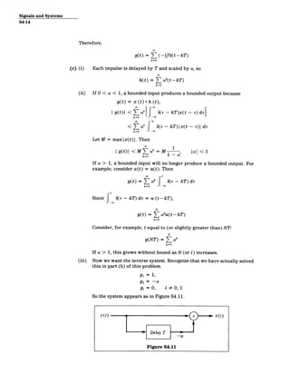
The given input in Figure S4.1-1 can be expressed as linear combinations of xi[n],
x 2[n], X3[n].
x,[n]
0 2
Figure S4.1-1
(a) x 4[n] = 2x 1 [n] - 2x 2[n] + x3[n]
(b) Using superposition, y 4[n] = 2yi[n] - 2y 2[n] + y3 [n], shown in Figure S4.1-2.
-1 0 1
Figure S4.1-2
(c) The system is not time-invariant because an input xi[n] + xi[n - 1] does not
produce an output yi[n] + yi[n - 1]. The input x,[n] + xi[n - 11 is xi[n] +
xi[n - 1] = x2[n] (shown in Figure S4.1-3), which we are told produces y 2[n].
Since y 2[n] # yi[n] + yi[n - 1], this system is not time-invariant.
x 1 [n] +x 1 [n-1] =x2[n]
n
0 1
Figure S4.1-3
S4-1](https://image.slidesharecdn.com/0a374ee9df1ba2a9cd985807c735afa6mitres6007s11hw04sol-230323105344-d3a7ef3f/85/convulution-1-320.jpg)
![4 Convolution
Solutions to
Recommended Problems
S4.1
The given input in Figure S4.1-1 can be expressed as linear combinations of xi[n],
x 2[n], X3[n].
x,[n]
0 2
Figure S4.1-1
(a) x 4[n] = 2x 1 [n] - 2x 2[n] + x3[n]
(b) Using superposition, y 4[n] = 2yi[n] - 2y 2[n] + y3 [n], shown in Figure S4.1-2.
-1 0 1
Figure S4.1-2
(c) The system is not time-invariant because an input xi[n] + xi[n - 1] does not
produce an output yi[n] + yi[n - 1]. The input x,[n] + xi[n - 11 is xi[n] +
xi[n - 1] = x2[n] (shown in Figure S4.1-3), which we are told produces y 2[n].
Since y 2[n] # yi[n] + yi[n - 1], this system is not time-invariant.
x 1 [n] +x 1 [n-1] =x2[n]
n
0 1
Figure S4.1-3
S4-1](https://image.slidesharecdn.com/0a374ee9df1ba2a9cd985807c735afa6mitres6007s11hw04sol-230323105344-d3a7ef3f/75/convulution-1-2048.jpg)
![Signals and Systems
S4-2
S4.2
The required convolutions are most easily done graphically by reflecting x[n] about
the origin and shifting the reflected signal.
(a) By reflecting x[n] about the origin, shifting, multiplying, and adding, we see
that y[n] = x[n] * h[n] is as shown in Figure S4.2-1.
(b) By reflecting x[n] about the origin, shifting, multiplying, and adding, we see
that y[n] = x[n] * h[n] is as shown in Figure S4.2-2.
y[n]
3
2
0 1 2 3 4 5 6
Figure S4.2-2
Notice that y[n] is a shifted and scaled version of h[n].
S4.3
(a) It is easiest to perform this convolution graphically. The result is shown in Fig
ure S4.3-1.](https://image.slidesharecdn.com/0a374ee9df1ba2a9cd985807c735afa6mitres6007s11hw04sol-230323105344-d3a7ef3f/85/convulution-2-320.jpg)
![Signals and Systems
S4-4
S4.4
(a) Since y[n] = E=-oox[m]h[n - m],
y[n] = 6
b[m - no]h[n - m] = h[n - no]
m= -oO
We note that this is merely a shifted version of h[n].
y [n] = h1[12 I
ae|41 8 n
(n 1) no (n1+ 1)
Figure S4.4-1
(b) y[n] = E =_c(!)'u[m]u[n m]
For n > 0: y[n] =
1 +
= 2( 1
y[n] = 2 - (i)"
Forn < 0: y[n] = 0
Here the identity
N-i N
_
T am
Mr=O 1 a
has been used.
y[n]
2--
140
0 1 2
Figure S4.4-2
(c) Reversing the role of the system and the input has no effect
because
y[n] = E x[m]h[n m] = L h[m]x[n m]
m=-oo
The output and sketch are identical to those in part (b).
,
on the output](https://image.slidesharecdn.com/0a374ee9df1ba2a9cd985807c735afa6mitres6007s11hw04sol-230323105344-d3a7ef3f/85/convulution-4-320.jpg)
![Signals and Systems
S4-6
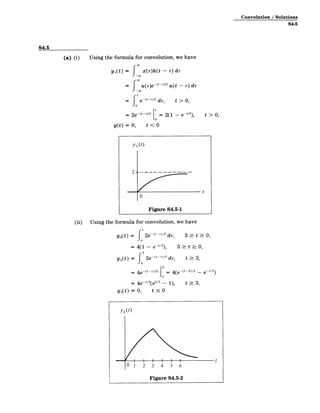
(b) Since x 2(t) = 2[xl(t) - xl(t - 3)] and the system is linear and time-invariant,
y2(t) = 2[yi(t) - y1(t - 3)].
For 0 s t s 3: y2(t) = 2yi(t) = 4(1 - e-'/2)
For 3 t y 2(t) = 2y,(t) - 2yi(t - 3)
= 4(1 - e-1/2 4(1 - e- t
-3)2)
= 4e- t/2
e
3
/
2
_ 1
Fort< 0: y2(t) = 0
We see that this result is identical to the result obtained in part (a)(ii).
Solutions to
Optional Problems
S4.6
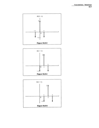
(a)
x(T)
1
T
0 1
Figure S4.6-1
h(-1 -r)
2,
-2 T
--
1 0
--1 '
Figure S4.6-2](https://image.slidesharecdn.com/0a374ee9df1ba2a9cd985807c735afa6mitres6007s11hw04sol-230323105344-d3a7ef3f/85/convulution-6-320.jpg)
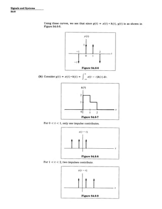
![Convolution / Solutions
S4-9
For 2 < t < 3, two impulses contribute.
x(t- r)
Figure S4.6-10
For 3 < t < 4, one impulse contributes.
t)
x(t
Figure S4.6-11
For t < 0 or t > 4, there is no contribution, so y(t) is as shown in Figure
S4.6-12.
y(t)
3 -
2
I-
U' 1 2 3 4
Figure S4.6-12
S4.7
y[n] = x[n] * h[n]
= 1 x[n - m]h[m]
nO
=- - n 0,
anmm, >
M=0](https://image.slidesharecdn.com/0a374ee9df1ba2a9cd985807c735afa6mitres6007s11hw04sol-230323105344-d3a7ef3f/85/convulution-9-320.jpg)
![Signals and Systems
S4-10
y[n] = a" = a" L (la)
a n+1 _ n+1
a - #
n > 0,
y[n] = 0, n < 0
S4.8
(a) x(t) = E_= - kT) is a series of impulses spaced T apart.
x(t)
t
-2T -T 0 T 2T
Figure S4.8-1
(b) Using the result x(t) *(t - to) = x(to), we have
y(t)
.. t
-2 3 -1 3
3
0 1 1 2
2 2 2 2
Figure S4.8-2
So y(t) = x(t) * h(t) is as shown in Figure S4.8-3.
y(t)
2
-2 -3 -1 -j 0 1 1 3 2
22 2 2
Figure S4.8-3](https://image.slidesharecdn.com/0a374ee9df1ba2a9cd985807c735afa6mitres6007s11hw04sol-230323105344-d3a7ef3f/85/convulution-10-320.jpg)
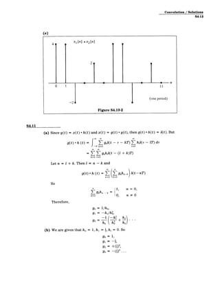
![Convolution / Solutions
S4-11
S4.9
(a) False. Counterexample: Let g[n] = b[n]. Then
x[n] * {h[n]g[n]} = x[n] h[0],
{x[n]* h[n]}g[n] = b[n] [x[n] *h[n]]
n=0
and x[n] may in general differ from b[n].
(b) True.
y(2t) = fx(2t - r)h(r)dr
Let r' = T/
2
. Then
y(2t) = f x(2t - 2r')h(2r')2dr'
= 2x(2t)* h(2t)
(c) True.
y(t) = x(t) * h(t)
y(- t) = x(-t) * h(-t)
-f x(-t + r)h(-r)dr = f [-x(t - r)][-h(r)] dT
=f x(t - r)h(r)dr since x(-) and h(-) are odd fu ictions
- y(t)
Hence y( t) = y(-t), and y(t) is even.
(d) False. Let
x(t) = b(t - 1)
h(t) = b(t + 1)
y(t) = b(t), Ev{ y (t)} = 6(t)
Then
x(t) *Ev{h(t)} =b(t - 1) *i[b(t + 1) + b(t - 1)]
= i[b(t) + b(t - 2)],
Ev{x(t)} * h(t) =1[6t - 1) + b(t + 1)] * b(t + 1)
= 1[b(t) + b(t + 2)]
But since 1[6(t - 2) + b(t + 2)] # 0,
Ev{y(t)} # x(t) *Ev{h(t)} + Ev{x(t)} *h(t)
S4.10
(a)
9(t) = Jro
TO21 (r)22(t - r) dr,
O
D(t + T0) = J 21 (T)- 2(t + To - r) d-r
= TO 1 (r) 2 (t - r)dr = (t)](https://image.slidesharecdn.com/0a374ee9df1ba2a9cd985807c735afa6mitres6007s11hw04sol-230323105344-d3a7ef3f/85/convulution-11-320.jpg)
![Signals and Systems
S4-12
(b)
9a(t) = T
a+TO
2 1(i)2 2(t - -) dr,
a
9a(t)
=
=
kTo + b, where 0
(k+1)T0+b
2 1(r)A 2(t - i)
kT0+b
TO+b
b -
dr,
To,
Pa(t) = fb 2 1 (i)± 2 (t - r) di, i' = i - b
FTo T70+b
= T1()- t - r) dr + 1&)2(t - r) di
2
b TO
Tb ()A - r) d1 2- ) di
= )
T)TO
= 21 )12( t T ) dr =q t )
t(-r
(c) For 0 s t - I
ft e- I
9(t) = di + Ti±e-'di
0e + e/2+t1/2+1
=(-e-' t + (-e-T
0 11/2+t)
(t) = 1 - e~' + e-(*±1/2) - e-1 = 1 - e-1 + (e 1/
2
- 1)e-
For s t < 1:
= ft
t(t) e-' di = e- ( 1/2) - e
- 1/2 )e
(d) Performing the periodic convolution graphically, we obtain the solution as
shown in Figure S4.10-1.
2 X1[n] *x2[n]
19
0 1 3 4 5
-16 (one period)
Figure S4.10-1](https://image.slidesharecdn.com/0a374ee9df1ba2a9cd985807c735afa6mitres6007s11hw04sol-230323105344-d3a7ef3f/85/convulution-12-320.jpg)
![Convolution / Solutions
S4-15
(d) If x[n] = 6[n], then y[n] = h[n]. If
x[n] = go[n] + iS[n-N],
then
y[n] = -h[n] + -h[n],
y[n] = h[n]
S4.12
(a) b[n] = #[n] - -4[n - 1],
x[n] = ( x[k][n - k] = ( x[k]Q([n - k] - -p[n - k - 1]),
k=-- k=--w
x[n] = E (x[k] - ix[k - 1])4[n- k]
k= -w
So ak = x[k] - lx[k - 1].
(b) If r[n] is the response to #[n], we can use superposition to note that if
x[n] = ( akp[n - k],
k=
then
y[n] = Z akr[n - k]
k= -w
and, from part (a),
y[n] = ( (x [k] - fx[k - 1])r[n - k]
k=
(c) y[n] = i/[n] *x[n] * r[n] when
[n] = b[n] - in- 1]
and, from above,
3[n] 4[n] - -[- 1]
So
/[n] = #[n] - -#[n - 11 - 1(#[n - 11 - -$[n - 2]),
0[n] = *[n] - *[n - 1] + {1[n - 2]
(d) 4[n] - r[n],
#[n - 1] - r[n - 1],
b[n] = 4[n] - -1[n- 1] - r[n] - fr[n -1]
So
h[n] = r[n] - tr[n -1],
where h[n] is the impulse response. Also, from part (c) we know that
y[n] = Q[n] *x[n] *r[n]
and if x[n] = #[n] produces r[n], it is apparent that #[n] * 4[n] = 6[n].](https://image.slidesharecdn.com/0a374ee9df1ba2a9cd985807c735afa6mitres6007s11hw04sol-230323105344-d3a7ef3f/85/convulution-15-320.jpg)


![Digital Signal Processing[ECEG-3171]-Ch1_L03](https://cdn.slidesharecdn.com/ss_thumbnails/dspl3-180427094423-thumbnail.jpg?width=640&height=640&fit=bounds)